library(ggplot2)
library(grid)

te_ink <- "#16241d"; te_forest <- "#275139"; te_gold <- "#c9b458"
te_rust <- "#b5534e"; te_sage <- "#93a87f"; te_line <- "#dad9ca"; te_muted <- "#5d6b61"

theme_te <- function() {
  theme_minimal(base_size = 12) +
    theme(
          plot.background  = element_rect(fill = "#f5f4ee", colour = NA),
          panel.background = element_rect(fill = "#f5f4ee", colour = NA),
          text = element_text(colour = te_ink),
          plot.title = element_text(face = "bold", colour = te_ink),
          plot.subtitle = element_text(colour = te_muted, size = rel(0.9)),
          axis.text = element_text(colour = te_muted),
          panel.grid.major = element_line(colour = te_line, linewidth = 0.3),
          panel.grid.minor = element_blank(),
          legend.position = "top", legend.title = element_blank())
}Jolly-Seber and POPAN: abundance from marks
R
capture-recapture
abundance
population ecology
ecology tutorial
Fit the Jolly-Seber superpopulation model by hand in base R, see where abundance comes from, and watch it collapse when first capture differs from recapture.
Corrected 7 October 2026: the post called trap response the single most common way capture probability varies in a real study; it now calls it one of the most common ways.
Corrected 30 September 2026: the post said that under trap response POPAN concludes it missed almost nobody; it now says that POPAN concludes it missed far fewer animals than it really did.
The Cormack-Jolly-Seber model gives you survival and nothing else. That is not a limitation anyone forgot to fix: it is the price of a deliberate move. CJS conditions on first capture, so the probability of getting marked in the first place never enters the likelihood. Animals you never caught contribute nothing, which is exactly why the model is safe, and exactly why it cannot count.
To count, you have to model the first capture. This post builds the Jolly-Seber superpopulation model (the POPAN parameterisation of Schwarz and Arnason) by hand, shows that it contains CJS unchanged, and then shows what the extra layer costs.
A world where we know the answer
Six capture occasions, a superpopulation of 400 animals that enter over time, apparent survival 0.80 between occasions, and a capture probability of 0.35 that is the same for every animal on every occasion. The entry probabilities put most of the population in at the start and trickle the rest in.
sim_js <- function(N, beta, phi, p, seed, pf = p) {
  set.seed(seed); k <- length(beta)
  e <- sample.int(k, N, replace = TRUE, prob = beta)
  Alive <- matrix(FALSE, N, k)
  Alive[cbind(seq_len(N), e)] <- TRUE
  for (t in 2:k) Alive[, t] <- Alive[, t] | (Alive[, t - 1] & runif(N) < phi)
  H <- matrix(0L, N, k); seen <- rep(FALSE, N)
  for (t in seq_len(k)) {
    H[, t] <- as.integer(Alive[, t] & runif(N) < ifelse(seen, p, pf))
    seen <- seen | H[, t] == 1L
  }
  list(H = H, Alive = Alive)
}

k <- 6; Nsup <- 400; phi <- 0.80; p <- 0.35
beta <- c(0.42, 0.14, 0.12, 0.12, 0.10, 0.10)
d <- sim_js(Nsup, beta, phi, p, seed = 4276)
H <- d$H
n_ever  <- sum(rowSums(H) > 0)
n_never <- sum(rowSums(H) == 0)
Ntrue   <- colSums(d$Alive)
ncount  <- colSums(H)
c(ever = n_ever, never = n_never)
ever never
260 140 260 animals were caught at least once. 140 were never caught at all, and every one of them is invisible to CJS by construction. The raw counts per occasion are 65, 74, 67, 68, 70, 70 against true sizes of 186, 202, 190, 188, 197, 207: the count recovers a fraction 0.354 of the truth, which is just p with sampling noise on top. A count is an abundance estimate multiplied by an unknown number. That is the problem to solve.
CJS first: the survival core
The CJS likelihood needs three numbers per animal: the occasion of first capture f, the occasion of last capture l, and the number of ticks s. Everything after the last capture is absorbed by chi, the probability of not being seen again given you were alive at l.
hsum <- function(H) {
  k <- ncol(H); idx <- col(H) * H; idx[idx == 0] <- NA
  list(f = suppressWarnings(apply(idx, 1, min, na.rm = TRUE)),
       l = suppressWarnings(apply(idx, 1, max, na.rm = TRUE)),
       s = rowSums(H), k = k)
}
chi_vec <- function(phi, p, k) {
  chi <- numeric(k); chi[k] <- 1
  for (j in (k - 1):1) chi[j] <- (1 - phi) + phi * (1 - p) * chi[j + 1]
  chi
}
cjs_nll <- function(par, S) {
  phi <- plogis(par[1]); p <- plogis(par[2]); chi <- chi_vec(phi, p, S$k)
  v <- -sum(log(phi^(S$l - S$f) * p^(S$s - 1) * (1 - p)^(S$l - S$f - S$s + 1) * chi[S$l]))
  if (!is.finite(v)) 1e10 else v
}
fit_cjs <- function(H) {
  S <- hsum(H[rowSums(H) > 0, , drop = FALSE])
  fit <- optim(c(qlogis(0.7), qlogis(0.3)), cjs_nll, S = S, method = "BFGS", hessian = TRUE)
  V <- tryCatch(solve(fit$hessian), error = function(e) matrix(NA, 2, 2))
  se <- sqrt(diag(V)); ph <- plogis(fit$par[1]); pd <- plogis(fit$par[2])
  list(phi = ph, p = pd, nll = fit$value,
       se_phi = se[1] * ph * (1 - ph), se_p = se[2] * pd * (1 - pd))
}
cj <- fit_cjs(H)
CJS returns apparent survival 0.7843 (SE 0.0346) against a true 0.80, and capture probability 0.3500 against a true 0.35. Both are fine. Neither is an abundance.
POPAN: one more layer
POPAN adds two things to the same machinery. First, a superpopulation size N: every animal that was ever alive and available during the study, caught or not. Second, entry probabilities beta, the fraction of that superpopulation joining at each occasion. The probability of a capture history then needs two new pieces: nu, the chance an animal entering at e is never caught at all, and an entry term summing over every occasion at which an animal could have arrived before its first capture. The N - n animals never seen enter the likelihood through a binomial coefficient and nu.
all_hist <- function(k) as.matrix(expand.grid(rep(list(0:1), k))[, k:1])

nu_vec <- function(phi, p, k) {
  nu <- numeric(k); nu[k] <- 1 - p
  for (e in (k - 1):1) nu[e] <- (1 - p) * ((1 - phi) + phi * nu[e + 1])
  nu
}
ent_vec <- function(phi, p, beta, k) {
  x <- phi * (1 - p); g <- numeric(k); g[1] <- beta[1]
  if (k > 1) for (f in 2:k) g[f] <- x * g[f - 1] + beta[f]
  g
}
popan_ph <- function(S, phi, p, beta) {
  k <- S$k; chi <- chi_vec(phi, p, k); g <- ent_vec(phi, p, beta, k)
  ok <- S$s > 0; out <- numeric(length(S$s))
  out[!ok] <- sum(beta * nu_vec(phi, p, k))
  f <- S$f[ok]; l <- S$l[ok]; s <- S$s[ok]
  out[ok] <- g[f] * p * phi^(l - f) * p^(s - 1) * (1 - p)^(l - f - s + 1) * chi[l]
  out
}
popan_nll <- function(par, freq, S, n) {
  k <- S$k
  N <- n + exp(par[1]); phi <- plogis(par[2]); p <- plogis(par[3])
  bl <- c(0, par[4:(k + 2)]); beta <- exp(bl) / sum(exp(bl))
  ph <- popan_ph(S, phi, p, beta)
  P0 <- ph[S$s == 0]
  if (!is.finite(P0) || P0 <= 0 || P0 >= 1) return(1e10)
  pv <- ph[S$s > 0]; if (any(!is.finite(pv)) || any(pv <= 0)) return(1e10)
  v <- -(lgamma(N + 1) - lgamma(N - n + 1) + (N - n) * log(P0) + sum(freq * log(pv)))
  if (!is.finite(v)) 1e10 else v
}
fit_popan <- function(H, k, hess = TRUE) {
  A <- all_hist(k); SA <- hsum(A)
  keyA <- apply(A, 1, paste, collapse = "")
  seen <- apply(H[rowSums(H) > 0, , drop = FALSE], 1, paste, collapse = "")
  n <- length(seen)
  freq <- as.integer(table(factor(seen, levels = keyA[SA$s > 0])))
  st <- c(log(0.5 * n), qlogis(0.7), qlogis(0.3), rep(0, k - 1))
  fit <- optim(st, popan_nll, freq = freq, S = SA, n = n, method = "BFGS",
               control = list(maxit = 5000, reltol = 1e-13), hessian = hess)
  N <- n + exp(fit$par[1]); phi <- plogis(fit$par[2]); p <- plogis(fit$par[3])
  bl <- c(0, fit$par[4:(k + 2)]); beta <- exp(bl) / sum(exp(bl))
  Nt <- numeric(k); Nt[1] <- N * beta[1]
  for (t in 2:k) Nt[t] <- Nt[t - 1] * phi + N * beta[t]
  seN <- NA_real_
  if (hess) {
    V <- tryCatch(solve(fit$hessian), error = function(e) NULL)
    if (!is.null(V) && all(diag(V) > 0)) seN <- exp(fit$par[1]) * sqrt(V[1, 1])
  }
  list(N = N, phi = phi, p = p, beta = beta, Nt = Nt, n = n, seN = seN)
}
po <- fit_popan(H, k)
po_lo <- po$N - 1.96 * po$seN; po_hi <- po$N + 1.96 * po$seN
The superpopulation estimate is 412.4 (SE 25.2), with a Wald interval of [362.9, 461.9] around a true 400. The per-occasion sizes follow from N, beta and phi by simple bookkeeping.
Now the part worth pausing on. Compare the survival estimate from the two fits:
phi_gap <- cj$phi - po$phi
sprintf("%.3e", phi_gap)
[1] "1.628e-05"The difference is \(1.628 \times 10^{-5}\). POPAN did not improve the survival estimate, refine it, or borrow strength for it. It reproduced it. All POPAN does is bolt a superpopulation layer onto an unchanged CJS core, and every new number it gives you (abundance, recruitment, entry) is bought with the one assumption CJS refused to make: that the first capture works like a recapture.
df_nt <- data.frame(
  occasion = rep(1:k, 3),
  value = c(Ntrue, po$Nt, ncount),
  kind = rep(c("true size", "POPAN estimate", "raw count"), each = k))
p_nt <- ggplot(df_nt, aes(occasion, value, colour = kind, shape = kind)) +
  geom_line(data = subset(df_nt, kind == "true size"), linewidth = 0.9) +
  geom_point(size = 3) +
  scale_colour_manual(values = c(`true size` = te_ink, `POPAN estimate` = te_forest,
                                 `raw count` = te_gold)) +
  scale_y_continuous(limits = c(0, 240)) +
  labs(title = "What each quantity is actually measuring",
       subtitle = "Six occasions, superpopulation of 400, capture probability 0.35",
       x = "Occasion", y = "Number of animals") +
  theme_te()
p_nt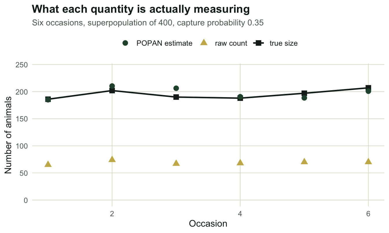
The honest limit: change the first capture only
Suppose animals react to being handled. A naive animal is caught with probability 0.20; once it has been through a trap, it is caught with probability 0.45. Nothing else changes: same survival, same entry, same superpopulation. This is trap response (also called a behavioural response to first capture), and it is one of the most common ways capture probability is not constant in a real study.
dt  <- sim_js(Nsup, beta, phi, 0.45, seed = 4276, pf = 0.20)
cjt <- fit_cjs(dt$H)
pot <- fit_popan(dt$H, k)
ratio_t <- pot$N / Nsup
CJS returns apparent survival 0.7864 (SE 0.0330), scattered around the truth by sampling noise rather than pulled off it. POPAN returns a superpopulation of 263.2, a ratio of 0.658 to the truth. Same data, same code, same animals. One estimate survives and the other does not.
One dataset is an anecdote, so take the noise out entirely. Feed the models expected frequencies rather than a simulated sample: enumerate all 64 possible histories, weight each by its exact probability under the trap-response world, and fit. What comes back is the probability limit, the number the estimator converges to with infinite data.
popan_ph2 <- function(S, phi, pf, p, beta) {
  k <- S$k
  chi <- chi_vec(phi, p, k)
  nu <- numeric(k); nu[k] <- 1 - pf
  for (e in (k - 1):1) nu[e] <- (1 - pf) * ((1 - phi) + phi * nu[e + 1])
  x <- phi * (1 - pf); g <- numeric(k); g[1] <- beta[1]
  if (k > 1) for (f in 2:k) g[f] <- x * g[f - 1] + beta[f]
  out <- numeric(length(S$s)); out[S$s == 0] <- sum(beta * nu)
  ok <- S$s > 0; f <- S$f[ok]; l <- S$l[ok]; s <- S$s[ok]
  out[ok] <- g[f] * pf * phi^(l - f) * p^(s - 1) * (1 - p)^(l - f - s + 1) * chi[l]
  out
}
cjs_nll_f <- function(par, S, fr) {
  phi <- plogis(par[1]); p <- plogis(par[2]); chi <- chi_vec(phi, p, S$k)
  v <- -sum(fr * log(phi^(S$l - S$f) * p^(S$s - 1) * (1 - p)^(S$l - S$f - S$s + 1) * chi[S$l]))
  if (!is.finite(v)) 1e10 else v
}
fit_cjs_f <- function(A, fr) {
  ok <- rowSums(A) > 0; S <- hsum(A[ok, , drop = FALSE])
  f <- optim(c(qlogis(.7), qlogis(.3)), cjs_nll_f, S = S, fr = fr[ok], method = "BFGS",
             control = list(reltol = 1e-14, maxit = 5000))
  list(phi = plogis(f$par[1]), p = plogis(f$par[2]))
}
fit_popan_f <- function(A, fr, n) {
  S <- hsum(A); k <- S$k
  f <- optim(c(log(0.5 * n), qlogis(.7), qlogis(.3), rep(0, k - 1)), popan_nll,
             freq = fr[S$s > 0], S = S, n = n, method = "BFGS",
             control = list(reltol = 1e-14, maxit = 8000))
  list(N = n + exp(f$par[1]), phi = plogis(f$par[2]), p = plogis(f$par[3]))
}

A <- all_hist(k); S <- hsum(A); M <- 1e6
exact_fit <- function(pf, pr) {
  ph <- popan_ph2(S, phi, pf, pr, beta); fr <- M * ph
  fc <- fit_cjs_f(A[S$s > 0, , drop = FALSE], fr[S$s > 0])
  fp <- fit_popan_f(A, fr, M * (1 - ph[S$s == 0]))
  list(phi = fc$phi, p = fc$p, ratio = fp$N / M, mass = sum(ph) - 1)
}
ex_ok <- exact_fit(0.35, 0.35)
ex_tr <- exact_fit(0.20, 0.45)
In the model-true world the limits are survival 0.800000, capture 0.350000, and a superpopulation ratio of 0.999999. Everything is where it should be, which tells us the machinery is right.
In the trap-response world, survival converges to 0.800000, still exactly the truth. Capture converges to 0.450000, which is exactly the recapture probability. Read that again: the model has not failed to fit. It has fitted the marked animals perfectly, and correctly reported the probability that governs them. Meanwhile the superpopulation converges to a ratio of 0.614025, an error of -38.60%.
The mechanism is not subtle once you see it. POPAN infers how many animals it missed from how hard the animals it has were to catch. In this world the animals it has are the easy ones (they have been caught before), so it concludes it missed far fewer animals than it really did. The never-caught animals were never caught because their capture probability was the low one, and no marked animal carries that number.
mc_popan <- function(gen, M = 200) {
  NN <- SE <- CV <- numeric(M)
  for (b in 1:M) {
    f <- fit_popan(gen(b)$H, k)
    NN[b] <- f$N; SE[b] <- f$seN
    CV[b] <- !is.na(f$seN) && abs(f$N - Nsup) < 1.96 * f$seN
  }
  list(N = NN, se = SE, cover = mean(CV))
}
mc_ok <- mc_popan(function(b) sim_js(Nsup, beta, phi, 0.35, seed = 30000 + b))
mc_tr <- mc_popan(function(b) sim_js(Nsup, beta, phi, 0.45, seed = 30000 + b, pf = 0.20))
Over 200 fresh datasets, the model-true world gives a mean estimate of 396.4 and a confidence interval that covers the truth 92.5% of the time, within Monte Carlo error of the nominal 95. The trap-response world gives a mean of 242.9, a bias of -157.1 animals, and coverage of 0.0%.
df_mc <- data.frame(N = c(mc_ok$N, mc_tr$N),
                    world = rep(c("model-true", "trap response"), each = 200))
ggplot(df_mc, aes(N, fill = world)) +
  geom_histogram(bins = 34, alpha = 0.75, position = "identity", colour = NA) +
  geom_vline(xintercept = Nsup, colour = te_ink, linetype = 2, linewidth = 0.8) +
  annotate("text", x = Nsup + 6, y = 30, label = "truth", colour = te_ink,
           hjust = 0, size = 3.6, fontface = "bold") +
  scale_fill_manual(values = c(`model-true` = te_forest, `trap response` = te_rust)) +
  labs(title = "Under trap response the interval never reaches the truth",
       subtitle = sprintf("200 studies per world; coverage %.1f per cent against %.1f per cent",
                          100 * mc_ok$cover, 100 * mc_tr$cover),
       x = "Estimated superpopulation size", y = "Studies") +
  theme_te()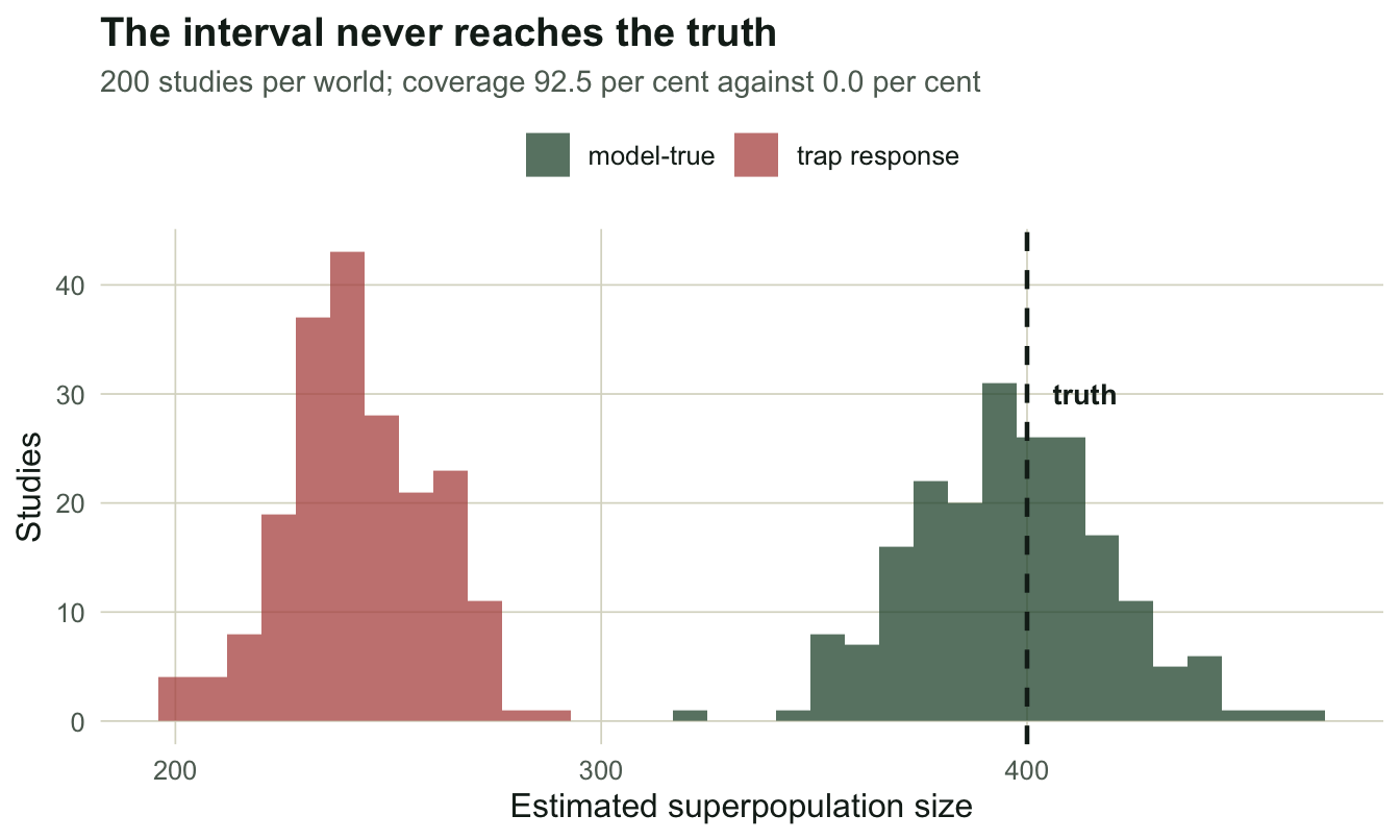
Zero per cent coverage is worth saying out loud. It does not mean the intervals are slightly optimistic. It means that across 200 studies, not one interval contained the right answer, and the reported standard error of about 14 animals was busy describing the precision of a number that was 157 animals wrong. Precision and accuracy are separate axes, and the likelihood only knows about the first.
What to take away
A count is an abundance multiplied by a detection probability you do not know. POPAN estimates that probability, which is a real achievement and lets you count. But it estimates it from the marked animals, and the number you need belongs to the unmarked ones. Whenever those two groups differ (handling shyness, trap happiness, different behaviour before and after marking), the survival estimate stays honest and the abundance quietly does not.
The remaining posts in this series take that observation apart. The seniority and lambda post shows that different quantities from the same data have graded exposure to this one assumption. The robust design post shows the design that buys back the missing information. And checking an open-population model asks the obvious question: could a goodness-of-fit test have warned us? The answer is worse than you might expect.
References
Jolly 1965 Biometrika 52(1-2):225-248 (10.1093/biomet/52.1-2.225)
Seber 1965 Biometrika 52(1-2):249-260 (10.1093/biomet/52.1-2.249)
Schwarz & Arnason 1996 Biometrics 52:860-873 (10.2307/2533048)
Pollock, Nichols, Brownie & Hines 1990 Wildlife Monographs 107:1-97
Link 2003 Biometrics 59(4):1123-1130 (10.1111/j.0006-341X.2003.00129.x)