Checking a survival model

Diagnostics for survival models: the proportional hazards test, martingale residuals for functional form, and Cox-Snell residuals for the distribution. Each detects a specific fault, and none proves the model right.

The last four posts fitted survival models: the Cox model, parametric and accelerated failure time models, the cumulative incidence function for competing risks, and frailty and recurrent-event models. Each rests on assumptions, and this post is about checking them: does the hazard ratio really stay constant over time, did you get the shape of a continuous covariate right, does the parametric distribution fit?

There are good, specific diagnostics for each of those questions. There is also a hard ceiling on what any of them can tell you, and the honest reading of a clean diagnostic is “no evidence against”, never “assumption verified”. This is the recurring lesson of every checking post on the blog, and it is at its sharpest here.

Does the hazard ratio hold over time

A Cox model claims one covariate multiplies the hazard by the same factor at every age. When the true effect fades or grows over time, that claim is false, and the standard tool to catch it is the scaled Schoenfeld residual and its test, cox.zph. A residual that trends against time is the signature of a time-varying effect.

To see it work, we build one covariate whose effect genuinely converges over time (data from a log-logistic accelerated failure time model, which gives non-proportional hazards) and one whose effect is genuinely constant (data from a Weibull proportional hazards model).

set.seed(4260)
n <- 400
x_np <- rbinom(n, 1, 0.5)
t_np <- exp(log(2) - 0.6 * x_np + 0.6 * qlogis(runif(n)))
o_np <- pmin(t_np, 3.5); d_np <- as.integer(t_np <= 3.5)
zph_np <- cox.zph(coxph(Surv(o_np, d_np) ~ x_np))

x_p <- rbinom(n, 1, 0.5); a <- 1.4; lam0 <- 2
t_p <- lam0 * exp(-log(2) * x_p / a) * (-log(runif(n)))^(1 / a)
o_p <- pmin(t_p, 4); d_p <- as.integer(t_p <= 4)
zph_p <- cox.zph(coxph(Surv(o_p, d_p) ~ x_p))

p_np <- zph_np$table["x_np", "p"]
p_p <- zph_p$table["x_p", "p"]

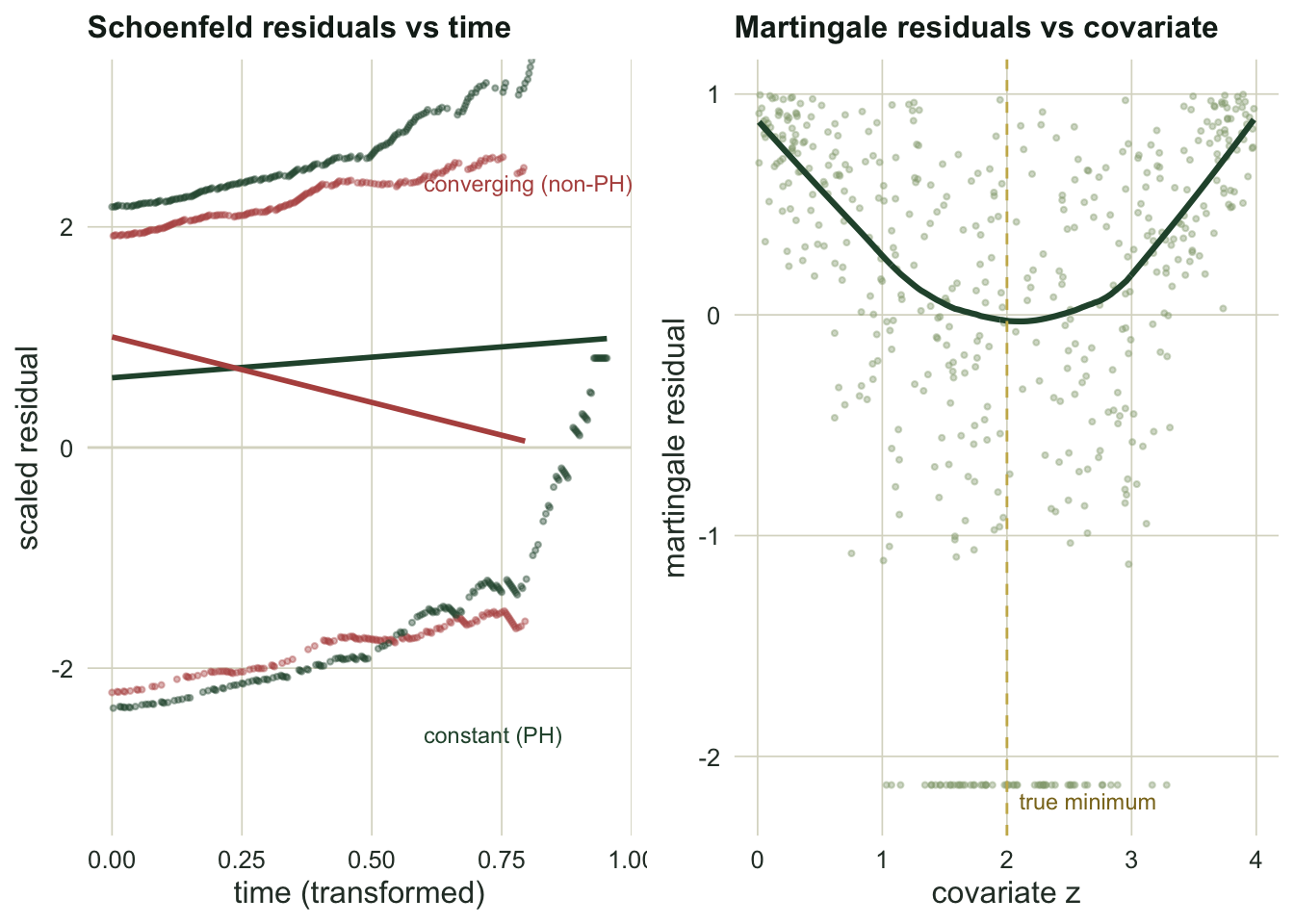
The test flags the converging covariate, with a proportional hazards p-value of 0.016, and clears the constant one, at 0.31. The residual plot below tells the same story visually: a downward slope for the non-proportional covariate, a flat cloud for the proportional one. When cox.zph fires, the usual fixes are stratifying on the offending variable or letting its coefficient vary with time.

set.seed(4261)
nb <- 500; z <- runif(nb, 0, 4)
t_b <- -log(runif(nb)) / (0.4 * exp(0.9 * (z - 2)^2))
o_b <- pmin(t_b, 3); d_b <- as.integer(t_b <= 3)
mart_null <- residuals(coxph(Surv(o_b, d_b) ~ 1), type = "martingale")
sm <- lowess(z, mart_null, f = 0.5)
z_min <- sm$x[which.min(sm$y)]
aic_lin <- AIC(coxph(Surv(o_b, d_b) ~ z))
aic_poly <- AIC(coxph(Surv(o_b, d_b) ~ poly(z, 2)))

Did you get the shape right

The second question is functional form: when a continuous covariate enters the hazard, a Cox model assumes it does so linearly on the log scale. Martingale residuals from a model with no covariates, plotted against the covariate, trace out its true shape. Here the covariate acts through a U-shape, low risk in the middle and high at both ends, and the smoother through the residuals recovers it, bottoming out at 2.11 against a true minimum at 2. Fitting the covariate as linear is badly wrong; adding a quadratic term drops the AIC from 4854.5 to 4552.8, a fall of 302.

`geom_smooth()` using formula = 'y ~ x'

Figure 1: Left: scaled Schoenfeld residuals against time. The converging covariate trends downward (its effect fades), the constant one is flat. Right: martingale residuals against a continuous covariate, with a smoother recovering the true U-shaped functional form.

Does the distribution fit

For a parametric model, the question is whether the assumed distribution matches the data. Cox-Snell residuals answer it: if the model fits, the residuals behave like a sample from a unit-exponential distribution, so their Nelson-Aalen cumulative hazard, plotted against the residual values, should follow the forty-five degree line. We reuse the log-logistic data from the parametric survival post and fit both the wrong distribution (Weibull) and the right one (log-logistic).

set.seed(4259)
nc <- 500; mu_c <- log(2.2); s_c <- 0.55
t_ll <- exp(mu_c + s_c * qlogis(runif(nc)))
cc <- 3.5; o_c <- pmin(t_ll, cc); d_c <- as.integer(t_ll <= cc)
fit_w  <- survreg(Surv(o_c, d_c) ~ 1, dist = "weibull")
fit_ll <- survreg(Surv(o_c, d_c) ~ 1, dist = "loglogistic")
cs_w  <- { a <- 1 / fit_w$scale;  l <- exp(coef(fit_w)[1]); (o_c / l)^a }
cs_ll <- { b <- 1 / fit_ll$scale; al <- exp(coef(fit_ll)[1]); log(1 + (o_c / al)^b) }
na_dev <- function(cs, d) {
  sf <- survfit(Surv(cs, d) ~ 1); H <- -log(pmax(sf$surv, 1e-8))
  max(abs(H - sf$time))
}
dev_w <- na_dev(cs_w, d_c); dev_ll <- na_dev(cs_ll, d_c)

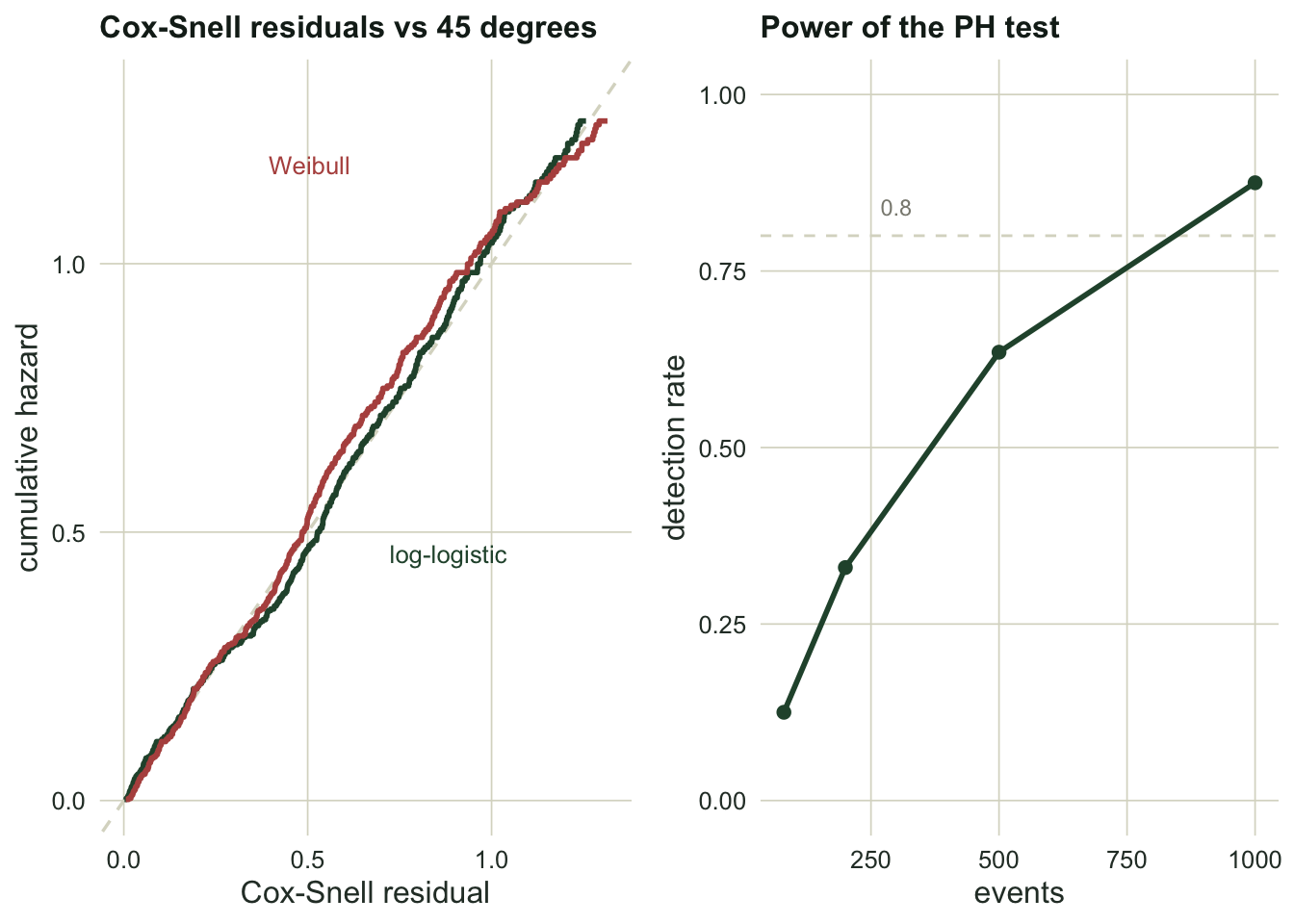
The correct model tracks the line more closely: the largest departure from forty-five degrees is 0.061 for the log-logistic against 0.081 for the Weibull. The gap is real but modest, and that caveat matters: with censoring the Cox-Snell check is a fairly blunt instrument; it will catch a badly wrong distribution but not split hairs between two plausible ones.

The two things a proportional hazards test cannot do

Now the ceiling. The proportional hazards test is neither a proof nor a disproof, and two short simulations show why.

First, a clean test does not prove proportionality; it may simply lack power. We generate genuinely non-proportional data and ask how often cox.zph detects it at various sample sizes.

power_zph <- function(nn, B = 200, seed = 7) {
  set.seed(seed); k <- 0
  for (b in 1:B) {
    x <- rbinom(nn, 1, 0.5); tt <- exp(log(2) - 0.6 * x + 0.6 * qlogis(runif(nn)))
    oo <- pmin(tt, 3.5); dd <- as.integer(tt <= 3.5)
    if (cox.zph(coxph(Surv(oo, dd) ~ x))$table["x", "p"] < 0.05) k <- k + 1
  }
  k / B
}
ns <- c(80, 200, 500, 1000)
pw <- sapply(ns, power_zph)

At 200 events the test finds the violation only 33 percent of the time, and even at 500 it misses roughly a third. A non-significant cox.zph on a modest data set is very weak evidence that hazards are proportional.

Second, a failed test does not prove the effect is time-varying; an omitted covariate can manufacture the appearance of non-proportionality. We generate data where two covariates both have strictly constant effects, then fit a model leaving one out.

set.seed(4262); B <- 250; flag_omit <- flag_full <- 0
for (b in 1:B) {
  nd <- 350; x1 <- rbinom(nd, 1, 0.5); x2 <- rnorm(nd)
  td <- lam0 * exp(-(log(2) * x1 + 1.5 * x2) / a) * (-log(runif(nd)))^(1 / a)
  od <- pmin(td, 4); dd <- as.integer(td <= 4)
  if (cox.zph(coxph(Surv(od, dd) ~ x1))$table["x1", "p"] < 0.05) flag_omit <- flag_omit + 1
  if (cox.zph(coxph(Surv(od, dd) ~ x1 + x2))$table["x1", "p"] < 0.05) flag_full <- flag_full + 1
}
rate_omit <- flag_omit / B; rate_full <- flag_full / B

With the strong covariate omitted, cox.zph flags the first covariate as non-proportional 16 percent of the time, far above the nominal five, even though its true effect never changes. Put the covariate back and the flag rate drops to 5 percent, where it belongs. The apparent time-varying effect was an artifact of unmodelled heterogeneity, not a real feature of the hazard.

Figure 2: Left: Cox-Snell residual cumulative hazard against the forty-five degree line; the log-logistic fit tracks it, the Weibull drifts away. Right: the power of the proportional hazards test to detect a genuine violation, low at small samples, so a clean test is weak evidence of proportionality.

What to take away

Survival models come with sharp, specific diagnostics, and you should run all of them. Use scaled Schoenfeld residuals and cox.zph for proportional hazards, martingale residuals for the functional form of a continuous covariate, and Cox-Snell residuals for a parametric distribution; for the frailty and recurrent-event models, the gap between the model-based and cluster-robust standard error is itself a check for unmodelled correlation, and for competing risks you would test the Fine-Gray proportional subdistribution hazards the same way. But read every result with the ceiling in mind. A clean proportional hazards test can simply lack power, and a failed one can be an omitted covariate in disguise. The diagnostics test the model you fit, not the question you care about, and the deepest assumptions, that competing events are handled correctly, that no important covariate is missing, that the sampled animals represent the population, are not checkable from the data at all. Run the checks, act on what they flag, and treat silence as the absence of evidence rather than evidence of correctness.

References

Cox, D. R. and Snell, E. J. (1968) A general definition of residuals. Journal of the Royal Statistical Society: Series B 30, 248-275. https://doi.org/10.1111/j.2517-6161.1968.tb00724.x

Grambsch, P. M. and Therneau, T. M. (1994) Proportional hazards tests and diagnostics based on weighted residuals. Biometrika 81, 515-526. https://doi.org/10.1093/biomet/81.3.515

Schoenfeld, D. (1982) Partial residuals for the proportional hazards regression model. Biometrika 69, 239-241. https://doi.org/10.1093/biomet/69.1.239

Therneau, T. M. and Grambsch, P. M. (2000) Modeling Survival Data: Extending the Cox Model. Springer. ISBN 978-0-387-98784-2.

Therneau, T. M., Grambsch, P. M. and Fleming, T. R. (1990) Martingale-based residuals for survival models. Biometrika 77, 147-160. https://doi.org/10.1093/biomet/77.1.147

Related tutorials

• Competing risks and cumulative incidence
• Parametric survival and the AFT model
• Frailty and recurrent event models
• Cox proportional hazards and the PH assumption

## References

Cox DR, Snell EJ 1968 Journal of the Royal Statistical Society: Series B 30:248-265 (10.1111/j.2517-6161.1968.tb00724.x)
Grambsch PM, Therneau TM 1994 Biometrika 81:515-526 (10.1093/biomet/81.3.515)
Schoenfeld D 1982 Biometrika 69:239-241 (10.1093/biomet/69.1.239)
Therneau TM, Grambsch PM 2000 Modeling Survival Data: Extending the Cox Model. Springer. ISBN 978-0-387-98784-2
Therneau TM, Grambsch PM, Fleming TR 1990 Biometrika 77:147-160 (10.1093/biomet/77.1.147)