Frailty and recurrent event models

Survival times that share a cluster or repeat within an individual are not independent. A naive model understates their uncertainty, and the correction is limited by the number of units, not events.

The Cox model and the parametric survival models both assume one row is one independent survival time. Field data rarely oblige. Littermates share a mother and a burrow; animals at one site share its predators and its weather; a single individual can be re-infected, re-captured, or breed again and again. Each of these breaks independence, and a model that ignores it reports standard errors that are too small, which turns into significance you have not earned.

This post covers the two standard fixes: a shared frailty for clustered survival, and the Andersen-Gill model for recurrent events. Both work with the survival package alone. And both carry the same honest limit: the correction is bounded by the number of independent units (clusters, or subjects), not by the number of events, so with few units even the corrected inference is shaky.

Clustered survival and shared frailty

Suppose 320 animals are spread across 40 sites, eight per site, and each site carries an unobserved level of risk shared by its residents, a frailty. We give each site a gamma-distributed frailty with variance one half, and two covariates: a site-level one (xb, say a habitat treatment applied to whole sites) and an individual one (xw, an animal trait). A shared frailty model adds the site as a random effect on the hazard.

set.seed(4258)
G <- 40; m <- 8; n <- G * m; theta <- 0.5
bW <- log(1.5); bB <- log(2.2); r0 <- 0.4
site <- rep(1:G, each = m)
z  <- rep(rgamma(G, shape = 1 / theta, rate = 1 / theta), each = m)
xb <- rep(rbinom(G, 1, 0.5), each = m)
xw <- rbinom(n, 1, 0.5)
u <- runif(n)
t_true <- -log(u) / (r0 * z * exp(bW * xw + bB * xb))
cens <- 5; obs <- pmin(t_true, cens); dead <- as.integer(t_true <= cens)

m_naive <- coxph(Surv(obs, dead) ~ xw + xb)
m_robust <- coxph(Surv(obs, dead) ~ xw + xb + cluster(site))
m_frailty <- coxph(Surv(obs, dead) ~ xw + xb + frailty(site, distribution = "gamma"))

se_n <- sqrt(diag(vcov(m_naive)))
se_r <- sqrt(diag(vcov(m_robust)))
theta_hat <- m_frailty$history[[1]]$theta
ratio_w <- se_r["xw"] / se_n["xw"]
ratio_b <- se_r["xb"] / se_n["xb"]

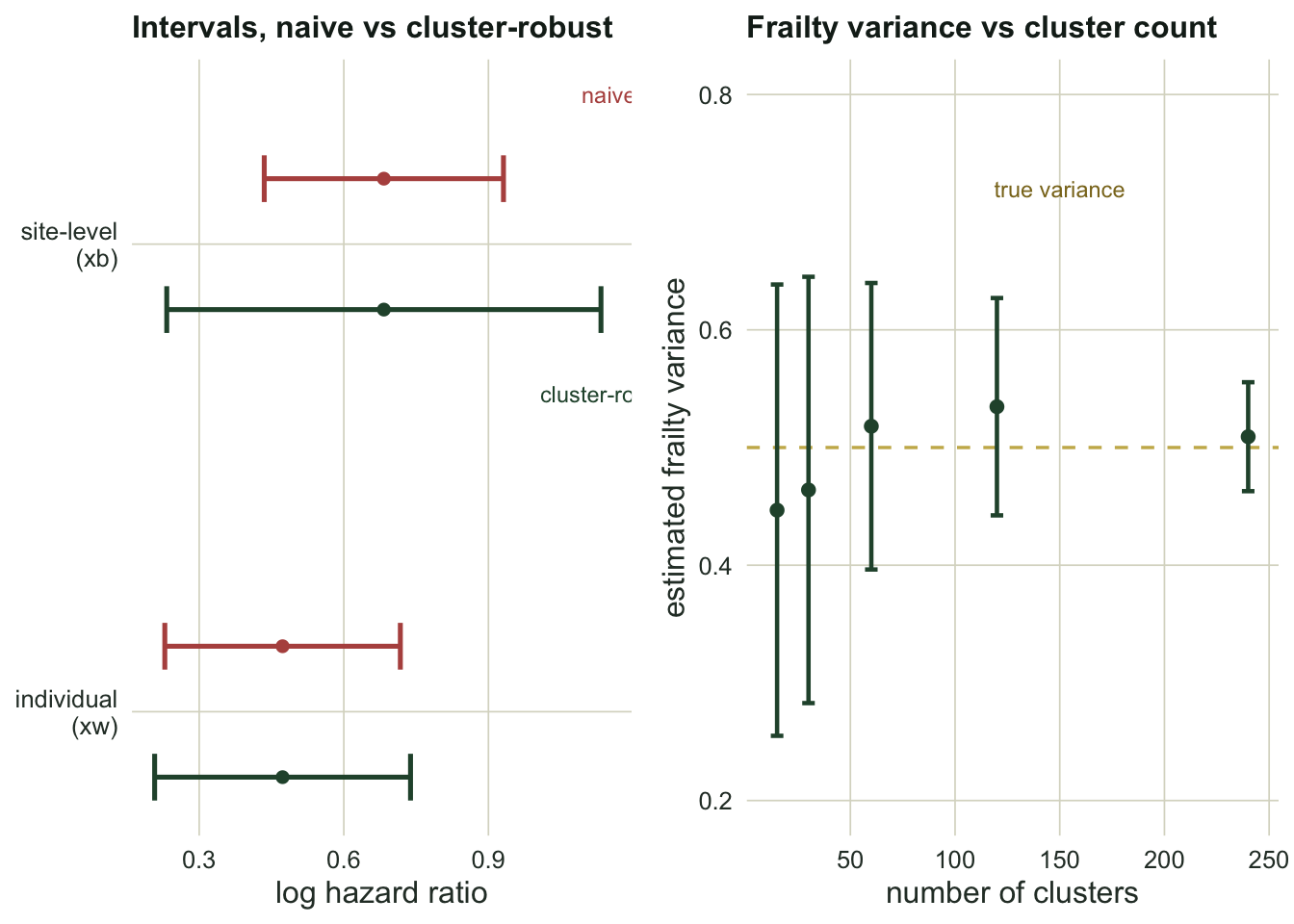
Ignoring the sites and adding a cluster-robust variance are two different fits, and the gap between them depends entirely on whether the covariate lives within a site or across sites. For the individual trait xw, the robust standard error is 1.09 times the naive one, essentially unchanged. For the site-level treatment xb, the robust standard error is 1.82 times the naive one, nearly double.

The reason is that a shared frailty affects everyone at a site together. When you compare two animals within the same site, the site frailty cancels, so an individual covariate is estimated from within-site contrasts that clustering barely touches. A site-level covariate has no within-site contrasts at all: its whole signal is the difference between sites, and there are only 40 of those, not 320. Ignore the clustering and you pretend you have 320 independent pieces of evidence about xb when you have closer to 40. The frailty model, fit separately, estimates a between-site variance of 0.63, confirming the sites really do differ.

A short coverage check makes the damage concrete: how often does a nominal 95 percent interval actually contain the true coefficient?

set.seed(42582); B <- 250
cov_nb <- cov_rb <- cov_nw <- cov_rw <- 0
for (b in 1:B) {
  zz <- rep(rgamma(G, shape = 1 / theta, rate = 1 / theta), each = m)
  xbb <- rep(rbinom(G, 1, 0.5), each = m); xww <- rbinom(n, 1, 0.5); uu <- runif(n)
  tt <- -log(uu) / (r0 * zz * exp(bW * xww + bB * xbb))
  oo <- pmin(tt, cens); dd <- as.integer(tt <= cens)
  cn <- coxph(Surv(oo, dd) ~ xww + xbb); cr <- coxph(Surv(oo, dd) ~ xww + xbb + cluster(site))
  vn <- sqrt(diag(vcov(cn))); vr <- sqrt(diag(vcov(cr)))
  if (abs(coef(cn)["xbb"] - bB) <= 1.96 * vn["xbb"]) cov_nb <- cov_nb + 1
  if (abs(coef(cr)["xbb"] - bB) <= 1.96 * vr["xbb"]) cov_rb <- cov_rb + 1
  if (abs(coef(cn)["xww"] - bW) <= 1.96 * vn["xww"]) cov_nw <- cov_nw + 1
  if (abs(coef(cr)["xww"] - bW) <= 1.96 * vr["xww"]) cov_rw <- cov_rw + 1
}

For the site-level covariate the naive interval covers the truth only 52 percent of the time, against a promised 95. The cluster-robust interval recovers most of that, at 84 percent, though with only 40 sites it stays a little short of nominal. For the individual covariate both are close to right (89 percent naive), because clustering never had much grip on it.

Warning: `geom_errorbarh()` was deprecated in ggplot2 4.0.0.
ℹ Please use the `orientation` argument of `geom_errorbar()` instead.

`height` was translated to `width`.

Figure 1: Left: 95 percent intervals from the naive and cluster-robust fits. For the site-level covariate the naive interval is far too narrow; for the individual covariate the two agree. Right: the estimated frailty variance is roughly unbiased on average but its spread across simulations shrinks only slowly with the number of clusters.

How much can you trust the frailty variance

The right panel above is a warning. Averaged over many simulations the frailty variance estimate sits close to its true value of one half at every cluster count, so it is not systematically biased. But the error bars, the spread of a single estimate, are wide when clusters are few: at 15 clusters the estimate’s standard deviation is 0.19, roughly 38 percent of the value being estimated, and it only tightens to 0.05 by 240 clusters. A single frailty variance from a handful of sites can land almost anywhere. Report it if you must, but do not build an argument on its exact size, and lean on the cluster-robust interval for the covariate effects.

Recurrent events

Now the other kind of dependence: one individual, many events. We follow 150 animals for five time units; each has its own event rate (a subject frailty, so events cluster within individuals) and a covariate. The naive habit is to keep only the first event per animal and run an ordinary Cox model. The Andersen-Gill model instead uses every event, in counting-process form: each animal contributes a sequence of start-stop intervals, each ending in an event or in censoring.

set.seed(4283)
N <- 150; tau <- 5; lam0 <- 0.6; bR <- log(1.6); phi <- 0.5
xi <- rbinom(N, 1, 0.5); wi <- rgamma(N, shape = 1 / phi, rate = 1 / phi)
lam_i <- lam0 * wi * exp(bR * xi)
rows <- list(); first_t <- first_s <- numeric(N)
for (i in 1:N) {
  t <- 0; ev <- numeric(0)
  repeat { t <- t + rexp(1, lam_i[i]); if (t > tau) break; ev <- c(ev, t) }
  if (length(ev) > 0) { first_t[i] <- ev[1]; first_s[i] <- 1 } else { first_t[i] <- tau; first_s[i] <- 0 }
  st <- c(0, ev); sp <- c(ev, tau); status <- c(rep(1, length(ev)), 0); keep <- sp > st
  rows[[i]] <- data.frame(id = i, start = st[keep], stop = sp[keep], status = status[keep], x = xi[i])
}
ag <- do.call(rbind, rows)
n_first <- sum(first_s); n_all <- sum(ag$status)

fit_first <- coxph(Surv(first_t, first_s) ~ xi)
fit_ag_naive <- coxph(Surv(start, stop, status) ~ x, data = ag)
fit_ag_robust <- coxph(Surv(start, stop, status) ~ x + cluster(id), data = ag)
se_first <- sqrt(vcov(fit_first))
se_ag_naive <- sqrt(vcov(fit_ag_naive))
se_ag_robust <- sqrt(fit_ag_robust$var)

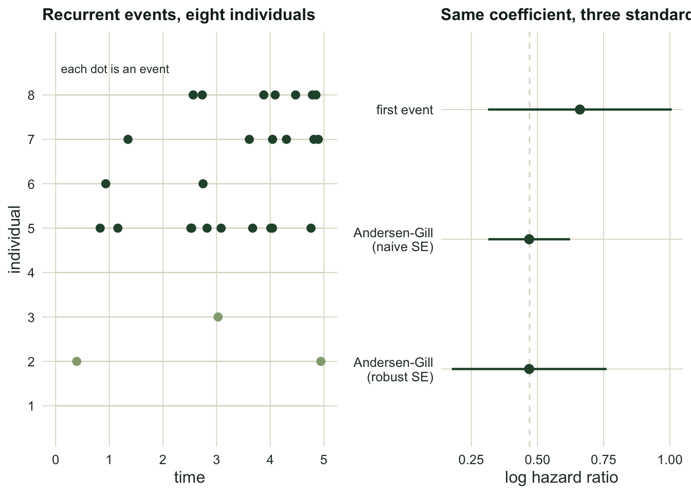
Keeping only first events uses 132 of the 665 events in the data. That looks wasteful, and it is, but the fix is not as generous as the event count suggests. The Andersen-Gill model with a naive standard error reports 0.079, less than half the first-event standard error of 0.177, which would imply the extra events bought a huge gain in precision. They did not. That naive standard error is wrong: it treats all 665 events as independent when they cluster within 150 animals. The robust (cluster) standard error, 0.149, is 1.89 times larger and tells the truth. Against the first-event analysis it is a genuine but modest improvement, 1.19 times narrower, not the 2.25 times the naive number pretended.

The lesson repeats: recurrent events add data, but positively correlated events within an individual carry less information than their count implies, and only the robust variance sees that. Always pair an Andersen-Gill fit with a cluster-robust standard error.

Figure 2: Left: event timelines for a sample of individuals, each with several events, showing why keeping only the first discards most of the data. Right: the coefficient interval from the first-event Cox model, the Andersen-Gill model with a naive standard error (far too narrow), and the Andersen-Gill model with a cluster-robust standard error (honest).

What to take away

Non-independent survival times need a model that says so. For clustered data, a shared frailty or a cluster-robust standard error stops you from overstating the significance of a covariate, but only for covariates that vary across clusters; within-cluster covariates were never much affected. For recurrent events, use the Andersen-Gill counting-process model with all events and a cluster-robust standard error, never the naive one, which mistakes correlated events for independent ones. Above all, remember what bounds the correction: the number of independent units. Forty sites give you about forty sites’ worth of information about a site-level effect no matter how many animals you tag, and a frailty variance from a handful of clusters is barely pinned down. When the units are few, report the effect with its honest interval and resist reading too much into the variance components.

References

Andersen, P. K. and Gill, R. D. (1982) Cox’s regression model for counting processes: a large sample study. Annals of Statistics 10, 1100-1120. https://doi.org/10.1214/aos/1176345976

Clayton, D. G. (1978) A model for association in bivariate life tables and its application in epidemiological studies of familial tendency in chronic disease incidence. Biometrika 65, 141-151. https://doi.org/10.1093/biomet/65.1.141

Lin, D. Y. and Wei, L. J. (1989) The robust inference for the Cox proportional hazards model. Journal of the American Statistical Association 84, 1074-1078. https://doi.org/10.1080/01621459.1989.10478874

Prentice, R. L., Williams, B. J. and Peterson, A. V. (1981) On the regression analysis of multivariate failure time data. Biometrika 68, 373-379. https://doi.org/10.1093/biomet/68.2.373

Therneau, T. M., Grambsch, P. M. and Pankratz, V. S. (2003) Penalized survival models and frailty. Journal of Computational and Graphical Statistics 12, 156-175. https://doi.org/10.1198/1061860031365

Vaupel, J. W., Manton, K. G. and Stallard, E. (1979) The impact of heterogeneity in individual frailty on the dynamics of mortality. Demography 16, 439-454. https://doi.org/10.2307/2061224

Related tutorials

• Competing risks and cumulative incidence
• Parametric survival and the AFT model
• Checking a survival model
• Nest survival with logistic exposure in R

## References

Andersen PK, Gill RD 1982 Annals of Statistics 10:1100-1120 (10.1214/aos/1176345976)
Clayton DG 1978 Biometrika 65:141-151 (10.1093/biomet/65.1.141)
Lin DY, Wei LJ 1989 Journal of the American Statistical Association 84:1074-1078 (10.1080/01621459.1989.10478874)
Prentice RL, Williams BJ, Peterson AV 1981 Biometrika 68:373-379 (10.1093/biomet/68.2.373)
Therneau TM, Grambsch PM, Pankratz VS 2003 Journal of Computational and Graphical Statistics 12:156-175 (10.1198/1061860031365)
Vaupel JW, Manton KG, Stallard E 1979 Demography 16:439-454 (10.2307/2061224)