---
title: "Parametric survival and the AFT model"
description: "A parametric survival model reads a covariate two ways, as a clock acceleration or a hazard ratio, and predicts absolute survival that Cox cannot give directly."
date: "2026-06-09 10:00"
date-modified: "2026-10-14"
categories: [R, survival analysis, ecology tutorial]
image: thumbnail.png
image-alt: "Two hazard curves over three years under the title Parametric survival: a dark green log-logistic curve that rises to a hump near two years and then eases, and a red Weibull curve that keeps rising, showing that the Weibull forces a monotone hazard."
---
*Corrected 14 October 2026: the post said the data cannot referee between the two tails because both distributions fit what was observed; the log-logistic fits better inside the observed range, and the text now says that the data bear on the tail only through that fit.*
The Cox model from the [proportional hazards tutorial](../cox-proportional-hazards/) leaves the baseline hazard unspecified and hands you a hazard ratio. That is often all you want. But sometimes you need the thing a hazard ratio cannot give: an actual survival time. How long does a collared animal live? What fraction survive two winters? A parametric survival model answers those directly, and it reads a covariate in a second, often more intuitive way, as a stretch or squeeze of the clock itself.
This post fits parametric survival models with `survreg`, shows how the accelerated failure time (AFT) and proportional hazards views are two readings of one Weibull fit, and then makes the case honestly: parametric models are not there to give you a tighter hazard ratio (the Cox model is nearly as efficient for that), they are there for the time-scale interpretation and for absolute survival predictions. The catch is that every prediction rests on the distribution you assumed, and the tail is the distribution's, not the data's.
```{r}
#| label: setup
#| message: false
#| warning: false
#| code-fold: true
#| code-summary: "Setup: packages, colours and plot theme"
library(ggplot2)
library(survival)
library(grid)

FOREST <- "#275139"; GOLD <- "#c9b458"; RUST <- "#b5534e"; SAGE <- "#93a87f"
INK <- "#16241d"; BODY <- "#2c3a31"; LINE <- "#dad9ca"

theme_te <- function() {
  theme_minimal(base_size = 12) +
    theme(plot.title = element_text(colour = INK, face = "bold", size = 12),
          plot.subtitle = element_text(colour = BODY, size = 10),
          axis.title = element_text(colour = BODY),
          axis.text = element_text(colour = BODY),
          legend.position = "none",
          panel.grid.minor = element_blank(),
          panel.grid.major = element_line(colour = LINE, linewidth = 0.3),
          plot.background = element_rect(fill = "#f5f4ee", colour = NA),
          panel.background = element_rect(fill = "#f5f4ee", colour = NA))
}
two_panel <- function(pa, pb) {
  grid.newpage(); pushViewport(viewport(layout = grid.layout(1, 2)))
  print(pa, vp = viewport(layout.pos.row = 1, layout.pos.col = 1))
  print(pb, vp = viewport(layout.pos.row = 1, layout.pos.col = 2))
}
haz_weib <- function(t, fit) { a <- 1 / fit$scale; l <- exp(coef(fit)[1]); (a / l) * (t / l)^(a - 1) }
haz_llog <- function(t, fit) { b <- 1 / fit$scale; al <- exp(coef(fit)[1]); ((b / al) * (t / al)^(b - 1)) / (1 + (t / al)^b) }
surv_weib <- function(t, fit) { a <- 1 / fit$scale; l <- exp(coef(fit)[1]); exp(-(t / l)^a) }
surv_llog <- function(t, fit) { b <- 1 / fit$scale; al <- exp(coef(fit)[1]); 1 / (1 + (t / al)^b) }
```
## One Weibull fit, two readings
Suppose we follow 400 animals whose deaths follow a Weibull distribution, and a habitat covariate `x` doubles the hazard (a true hazard ratio of two). We fit a Weibull model with `survreg`.
```{r}
#| label: fit-a
set.seed(4257)
n <- 400; shape_true <- 1.5; scale0 <- 2; log_hr_true <- log(2)
x <- rbinom(n, 1, 0.5)
u <- runif(n)
t_true <- scale0 * exp(-log_hr_true * x / shape_true) * (-log(u))^(1 / shape_true)
cens <- 3.0
obs <- pmin(t_true, cens); dead <- as.integer(t_true <= cens)

wb <- survreg(Surv(obs, dead) ~ x, dist = "weibull")
b_aft <- coef(wb)["x"]; sigma <- wb$scale
accel <- exp(b_aft)
weib_shape <- 1 / sigma
weib_hr <- exp(-b_aft / sigma)

V <- vcov(wb)
ib <- which(names(coef(wb)) == "x"); ils <- which(rownames(V) == "Log(scale)")
grad <- c(-1 / sigma, b_aft / sigma)
se_loghr_w <- sqrt(as.numeric(t(grad) %*% V[c(ib, ils), c(ib, ils)] %*% grad))
weib_hr_ci <- exp(log(weib_hr) + c(-1, 1) * 1.96 * se_loghr_w)

cox <- coxph(Surv(obs, dead) ~ x)
cox_hr <- exp(coef(cox)); cox_hr_ci <- exp(confint(cox))
```
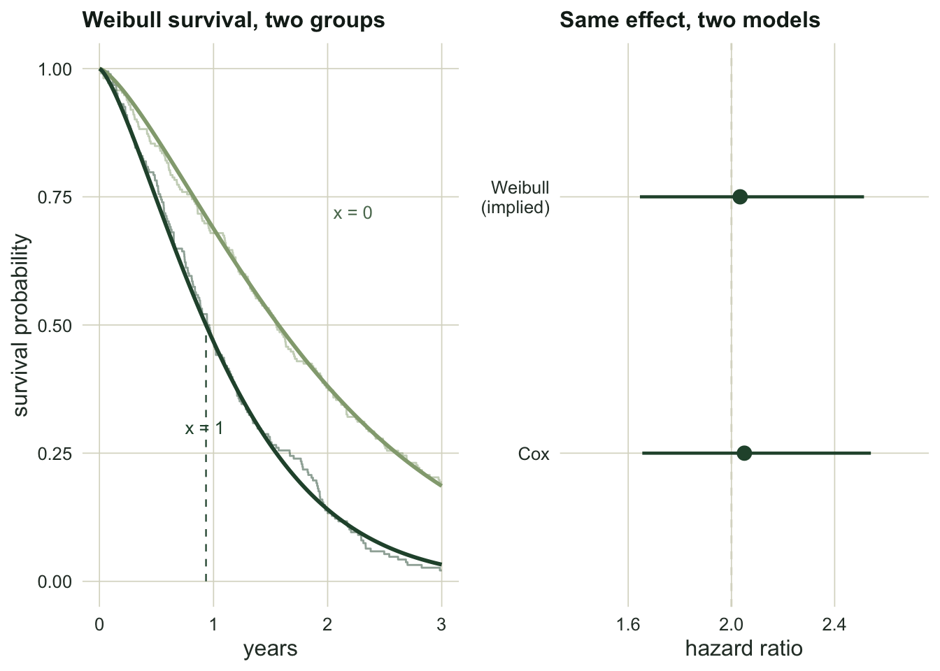
The Weibull fit has a shape of `r sprintf("%.2f", weib_shape)` (the truth is `r sprintf("%.1f", shape_true)`), so the hazard rises with age. Its covariate coefficient reads two ways. As an *accelerated failure time* effect, `exp` of the coefficient is `r sprintf("%.3f", accel)`: an animal in this habitat runs through its life on a clock compressed to about `r sprintf("%.0f", 100 * accel)` per cent of the baseline, so it dies sooner. As a *proportional hazards* effect, the same fit implies a hazard ratio of `r sprintf("%.2f", weib_hr)` (95 per cent interval `r sprintf("%.2f", weib_hr_ci[1])` to `r sprintf("%.2f", weib_hr_ci[2])`).
The Cox model, fit to the same data, gives a hazard ratio of `r sprintf("%.2f", cox_hr)` (interval `r sprintf("%.2f", cox_hr_ci[1])` to `r sprintf("%.2f", cox_hr_ci[2])`). The two agree, as they must when the proportional hazards assumption holds: the Weibull is the one distribution that is simultaneously an accelerated failure time model and a proportional hazards model, so its acceleration factor and its hazard ratio are locked together by the shape.
## What the parametric model buys, and what it does not
The acceleration reading is often the one an ecologist wants, because it lives on the time axis. And unlike Cox, a parametric fit predicts absolute survival directly.
```{r}
#| label: predict-a
med <- predict(wb, data.frame(x = c(0, 1)), type = "quantile", p = 0.5)
med_ratio <- med[2] / med[1]
```
Median survival is `r sprintf("%.2f", med[1])` years at `x` equal to zero and `r sprintf("%.2f", med[2])` years at `x` equal to one. Their ratio, `r sprintf("%.3f", med_ratio)`, is exactly the acceleration factor: an AFT model shrinks every quantile of the survival distribution by the same factor, which is what "accelerated" means. A Cox model cannot report either median without a separate, and rougher, estimate of the baseline hazard.
What the parametric model does *not* buy is a sharper hazard ratio. It is tempting to think that assuming the correct distribution must beat the Cox model on efficiency, but for the regression coefficient the Cox partial likelihood is already close to fully efficient. A short simulation makes the point across a wide range of censoring.
```{r}
#| label: efficiency-b
eff_ratio <- function(cens_at, B = 300, seed = 1) {
  set.seed(seed); cl <- wl <- cf <- numeric(B)
  for (b in 1:B) {
    xx <- rbinom(n, 1, 0.5); uu <- runif(n)
    tt <- scale0 * exp(-log_hr_true * xx / shape_true) * (-log(uu))^(1 / shape_true)
    ob <- pmin(tt, cens_at); dd <- as.integer(tt <= cens_at); cf[b] <- mean(1 - dd)
    ww <- survreg(Surv(ob, dd) ~ xx, dist = "weibull")
    cl[b] <- coef(coxph(Surv(ob, dd) ~ xx)); wl[b] <- -coef(ww)["xx"] / ww$scale
  }
  c(cens = mean(cf), cox_sd = sd(cl), weib_sd = sd(wl), ratio = sd(wl) / sd(cl))
}
eff_light <- eff_ratio(3.0, seed = 300)
eff_heavy <- eff_ratio(0.55, seed = 55)
```
At light censoring (`r sprintf("%.0f", 100 * eff_light["cens"])` per cent censored) the standard deviation of the Weibull log hazard ratio is `r sprintf("%.2f", eff_light["ratio"])` times the Cox one. At heavy censoring (`r sprintf("%.0f", 100 * eff_heavy["cens"])` per cent censored) the ratio is still `r sprintf("%.2f", eff_heavy["ratio"])`. The correct parametric model is not meaningfully more efficient for the covariate effect; the Cox model gives up almost nothing by refusing to name a distribution. Choose a parametric model for the time-scale interpretation and for absolute predictions, not for a tighter interval on the effect.
```{r}
#| label: fig-aft
#| echo: false
#| fig-cap: "Left: the Weibull fit gives smooth survival curves for each group, tracking the Kaplan-Meier estimates, with the median marked for the high-hazard group. Right: the Weibull-implied hazard ratio and the Cox hazard ratio agree, with essentially the same width, since the correct parametric model is not more efficient for the coefficient."
#| fig-alt: "Left panel, two parametric survival curves for the covariate groups overlaid on Kaplan-Meier step curves, with the earlier median marked for the high-hazard group. Right panel, two nearly identical hazard-ratio point-and-interval estimates near two."
km <- survfit(Surv(obs, dead) ~ x)
km_df <- data.frame(time = km$time, surv = km$surv,
grp = rep(c("x = 0", "x = 1"), km$strata))
tg <- seq(0, 3, length = 200)
lam0 <- exp(coef(wb)[1]); lam1 <- exp(coef(wb)[1] + coef(wb)["x"]); aa <- 1 / sigma
par_df <- rbind(
data.frame(time = tg, surv = exp(-(tg / lam0)^aa), grp = "x = 0"),
data.frame(time = tg, surv = exp(-(tg / lam1)^aa), grp = "x = 1"))
p1 <- ggplot() +
geom_step(data = km_df, aes(time, surv, colour = grp), linewidth = 0.5, alpha = 0.5) +
geom_line(data = par_df, aes(time, surv, colour = grp), linewidth = 1) +
geom_segment(aes(x = med[2], xend = med[2], y = 0, yend = 0.5), colour = FOREST, linetype = "dashed", linewidth = 0.4) +
scale_colour_manual(values = c("x = 0" = SAGE, "x = 1" = FOREST)) +
annotate("text", x = 2.05, y = 0.72, label = "x = 0", colour = "#5d7a5f", hjust = 0, size = 3.4) +
annotate("text", x = 0.88, y = 0.30, label = "x = 1", colour = FOREST, hjust = 1, size = 3.4) +
labs(title = "Weibull survival, two groups", x = "years", y = "survival probability") +
coord_cartesian(ylim = c(0, 1)) + theme_te()
fr <- data.frame(model = factor(c("Weibull\n(implied)", "Cox"), levels = c("Cox", "Weibull\n(implied)")),
hr = c(weib_hr, cox_hr),
lo = c(weib_hr_ci[1], cox_hr_ci[1]), hi = c(weib_hr_ci[2], cox_hr_ci[2]))
p2 <- ggplot(fr, aes(hr, model)) +
geom_vline(xintercept = 2, colour = LINE, linewidth = 0.5, linetype = "dashed") +
geom_pointrange(aes(xmin = lo, xmax = hi), colour = FOREST, linewidth = 0.8, size = 0.6) +
labs(title = "Same effect, two models", x = "hazard ratio", y = NULL) +
coord_cartesian(xlim = c(1.4, 2.7)) + theme_te()
two_panel(p1, p2)
```
## When the distribution is wrong
The Weibull hazard is monotone: once you assume it, the hazard can only rise or only fall with age. Real hazards are often hump-shaped, high just after a transition, then easing. Here we simulate log-logistic survival times, whose hazard rises then falls, and fit three distributions.
```{r}
#| label: fit-c
set.seed(4259)
nc <- 500; mu_c <- log(2.2); s_c <- 0.55
t_ll <- exp(mu_c + s_c * qlogis(runif(nc)))
cc <- 3.5
obs_c <- pmin(t_ll, cc); dead_c <- as.integer(t_ll <= cc)

fit_w  <- survreg(Surv(obs_c, dead_c) ~ 1, dist = "weibull")
fit_ll <- survreg(Surv(obs_c, dead_c) ~ 1, dist = "loglogistic")
fit_ln <- survreg(Surv(obs_c, dead_c) ~ 1, dist = "lognormal")
aic <- c(weibull = AIC(fit_w), loglogistic = AIC(fit_ll), lognormal = AIC(fit_ln))
best <- names(which.min(aic))
tg2 <- seq(0.05, 3, length = 200)
hump_peak <- tg2[which.max(haz_llog(tg2, fit_ll))]
```
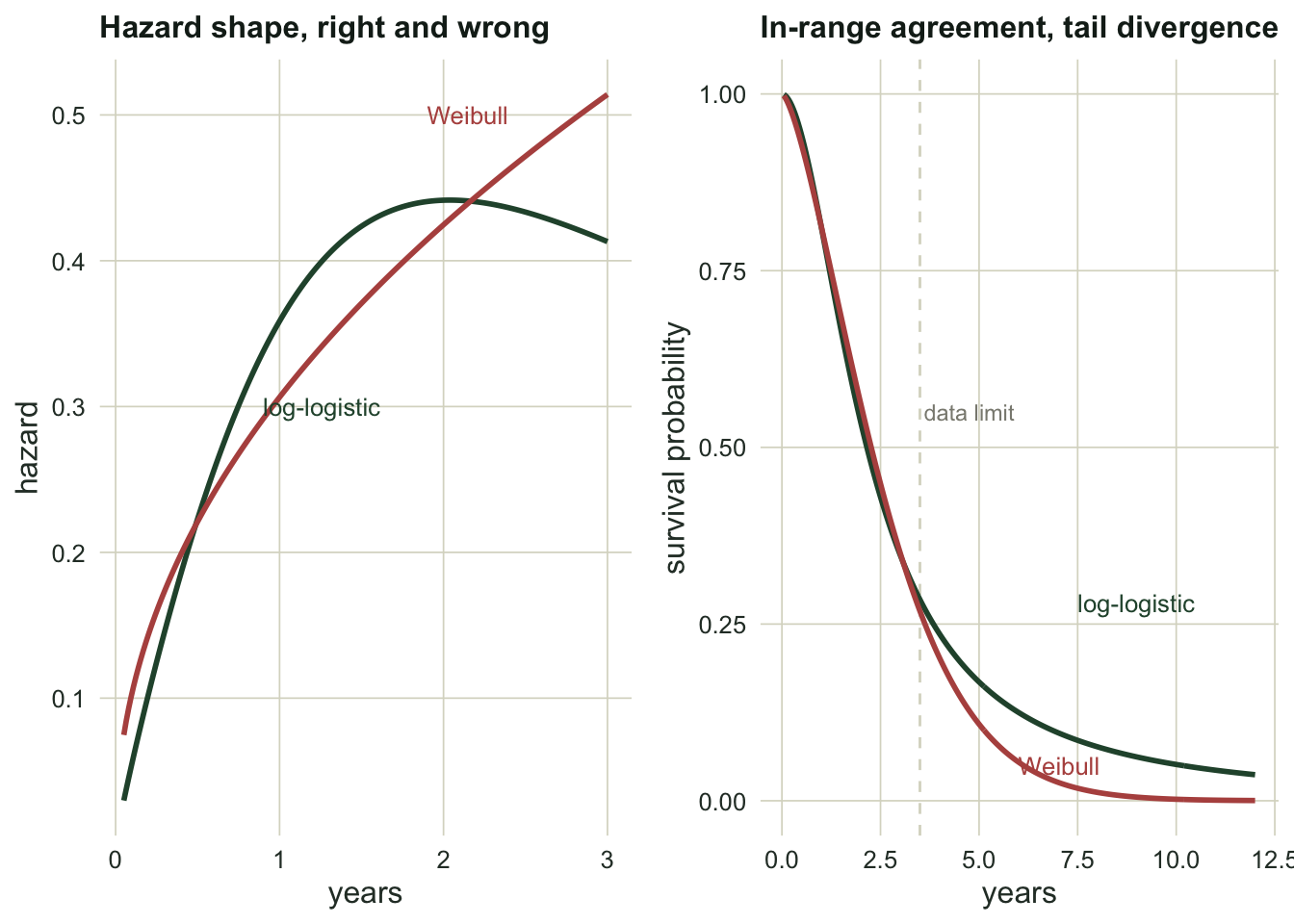
The AIC prefers the log-logistic (`r sprintf("%.1f", aic["loglogistic"])`) over the Weibull (`r sprintf("%.1f", aic["weibull"])`) and the log-normal (`r sprintf("%.1f", aic["lognormal"])`). The reason is the hazard shape: the log-logistic hazard climbs to a peak near `r sprintf("%.1f", hump_peak)` years and then declines, while the Weibull, forced to be monotone, simply keeps rising and never sees the hump. Fit the wrong distribution and you read the hazard backwards at the older ages: the Weibull says risk is still climbing where it is actually falling.
```{r}
#| label: fig-hazard
#| echo: false
#| fig-cap: "Left: on log-logistic data the true hazard is hump-shaped; the log-logistic fit recovers it, while the Weibull fit is forced to rise monotonically. Right: the two fitted survival curves agree over the range of the data (vertical line) but diverge sharply in the extrapolated tail."
#| fig-alt: "Left panel, a rising-then-falling log-logistic hazard against a monotonically rising Weibull hazard. Right panel, two survival curves nearly identical up to the data limit then separating, the log-logistic staying higher in the tail."
haz_df <- rbind(
data.frame(time = tg2, h = haz_weib(tg2, fit_w), what = "Weibull"),
data.frame(time = tg2, h = haz_llog(tg2, fit_ll), what = "log-logistic"))
p3 <- ggplot(haz_df, aes(time, h, colour = what)) +
geom_line(linewidth = 1) +
scale_colour_manual(values = c("Weibull" = RUST, "log-logistic" = FOREST)) +
annotate("text", x = 1.9, y = 0.50, label = "Weibull", colour = RUST, hjust = 0, size = 3.4) +
annotate("text", x = 0.9, y = 0.30, label = "log-logistic", colour = FOREST, hjust = 0, size = 3.4) +
labs(title = "Hazard shape, right and wrong", x = "years", y = "hazard") +
theme_te()
tg3 <- seq(0.05, 12, length = 300)
surv_df <- rbind(
data.frame(time = tg3, s = surv_weib(tg3, fit_w), what = "Weibull"),
data.frame(time = tg3, s = surv_llog(tg3, fit_ll), what = "log-logistic"))
p4 <- ggplot(surv_df, aes(time, s, colour = what)) +
geom_vline(xintercept = cc, colour = LINE, linewidth = 0.5, linetype = "dashed") +
geom_line(linewidth = 1) +
scale_colour_manual(values = c("Weibull" = RUST, "log-logistic" = FOREST)) +
annotate("text", x = 3.6, y = 0.55, label = "data limit", colour = "#8a8a80", hjust = 0, size = 3.1) +
annotate("text", x = 7.5, y = 0.28, label = "log-logistic", colour = FOREST, hjust = 0, size = 3.4) +
annotate("text", x = 6.0, y = 0.05, label = "Weibull", colour = RUST, hjust = 0, size = 3.4) +
labs(title = "In-range agreement, tail divergence", x = "years", y = "survival probability") +
theme_te()
two_panel(p3, p4)
```
## The tail belongs to the distribution
The right panel above carries the honest limit of the whole enterprise. Inside the range of the data the Weibull and log-logistic survival curves are almost indistinguishable, and their median survival estimates nearly match.
```{r}
#| label: tail-c
qs <- c(0.5, 0.9, 0.95)
q_w  <- predict(fit_w,  data.frame(z = 1)[1, , drop = FALSE], type = "quantile", p = qs)
q_ll <- predict(fit_ll, data.frame(z = 1)[1, , drop = FALSE], type = "quantile", p = qs)
tail_gap <- q_ll[3] - q_w[3]
```
The median survival is `r sprintf("%.2f", q_w[1])` years under the Weibull and `r sprintf("%.2f", q_ll[1])` under the log-logistic. But ask for the ninety-fifth percentile, the age only the longest-lived reach, and the Weibull says `r sprintf("%.2f", q_w[3])` years while the log-logistic says `r sprintf("%.2f", q_ll[3])`, a gap of `r sprintf("%.1f", tail_gap)` years. The data bear on this only through the fit inside the observed range, where the two survival curves are close and the log-logistic fits better; the difference itself lives entirely in a region no animal in the study reached. AIC picks the better fit among your candidates, but it cannot certify a tail beyond the last event.
## What to take away
A parametric survival model reads a covariate as an acceleration factor on the time scale (often the more natural reading in ecology) and, for the Weibull, equivalently as a hazard ratio; predict median survival and survival probabilities directly, which a Cox model cannot. Do not reach for a parametric model expecting a tighter hazard ratio, because the Cox model is nearly as efficient for the coefficient at any level of censoring. Choose the distribution by fitting a few candidates and comparing them (AIC, and a look at the fitted hazard shape against a flexible baseline), remembering that the log-logistic and log-normal allow the hump-shaped hazards the Weibull forbids. And treat every extrapolation past the last observed death as a property of the distribution you assumed, not a fact the data delivered.
## References
Bennett S 1983 Statistics in Medicine 2(2):273-277 (10.1002/sim.4780020223)
Cox DR 1972 Journal of the Royal Statistical Society: Series B 34(2):187-202 (10.1111/j.2517-6161.1972.tb00899.x)
Kalbfleisch JD, Prentice RL 2002 The Statistical Analysis of Failure Time Data, 2nd edition. Wiley. ISBN 978-0-471-36357-6
Muenchow G 1986 Ecology 67(1):246-250 (10.2307/1938524)
Therneau TM, Grambsch PM 2000 Modeling Survival Data: Extending the Cox Model. Springer. ISBN 978-0-387-98784-2
Wei LJ 1992 Statistics in Medicine 11(14-15):1871-1879 (10.1002/sim.4780111409)
## Related tutorials
- [Competing risks and cumulative incidence](../competing-risks-cumulative-incidence/)
- [Fire return intervals from a short scar record](../fire-return-intervals-from-fire-scars/)
- [Checking a survival model](../checking-a-survival-model/)
- [Interval-censored survival from visit data](../interval-censored-survival/)