Cox proportional hazards and the PH assumption

Fit a Cox proportional hazards model in R, read the hazard ratios, test the proportional-hazards assumption with Schoenfeld residuals, and stratify to fix it.

The Kaplan-Meier estimator compares survival between a few groups but cannot adjust for a continuous covariate or hold several predictors constant at once. The Cox proportional hazards model does both. It relates the hazard, the instantaneous risk of the event, to covariates without committing to a shape for the baseline hazard, which makes it the workhorse of survival analysis in ecology and everywhere else. The price of that flexibility is one assumption: each covariate multiplies the hazard by a constant factor that does not change over time. This post fits a Cox model in base R with the recommended survival package, interprets the hazard ratios, and then spends most of its length on the assumption, because a hazard ratio quoted from a model that violates it is a single number standing in for an effect that actually reverses.

Survival data with covariates

The example follows 220 tagged individuals to death or censoring, each carrying two covariates: a standardised parasite load, and a life stage, juvenile or adult. Parasite load is built to act proportionally, raising the hazard by a fixed multiple. Stage is built to violate that rule: juveniles start at high risk that eases as they grow, adults start safe and become frailer, so the two hazards cross rather than staying in fixed ratio.

library(survival)
library(ggplot2)
library(dplyr)

te_ink <- "#16241d"; te_body <- "#2c3a31"; te_forest <- "#275139"
te_label <- "#46604a"; te_sage <- "#93a87f"; te_paper <- "#f5f4ee"
te_line <- "#dad9ca"; te_gold <- "#c9b458"; te_deep <- "#1d5b4e"
te_brick <- "#b5534e"; te_faint <- "#5d6b61"
theme_te <- function(base_size = 12) {
  theme_minimal(base_size = base_size) +
    theme(text = element_text(colour = te_body),
          plot.title = element_text(colour = te_ink, face = "bold"),
          plot.subtitle = element_text(colour = te_faint),
          axis.title = element_text(colour = te_label),
          axis.text = element_text(colour = te_body),
          panel.grid.minor = element_blank(),
          panel.grid.major = element_line(colour = te_line, linewidth = 0.3),
          plot.background = element_rect(fill = te_paper, colour = NA),
          panel.background = element_rect(fill = te_paper, colour = NA),
          legend.background = element_rect(fill = te_paper, colour = NA),
          legend.position = "none")
}

set.seed(414)
n <- 220
parasite <- round(rnorm(n), 3)                        # standardised parasite load
stage <- factor(sample(c("Juvenile", "Adult"), n, replace = TRUE))
shape <- ifelse(stage == "Juvenile", 0.85, 1.75)      # different shape => non-proportional
scale <- 26 * exp(-0.45 * parasite)                   # higher load => shorter life (proportional)
tt <- rweibull(n, shape = shape, scale = scale)
ct <- pmin(rexp(n, 1 / 70), 42)                       # loss to follow-up plus admin end
time <- pmin(tt, ct); status <- as.integer(tt <= ct)
d <- data.frame(time = round(time, 2), status = status, parasite = parasite, stage = stage)
c(n = n, events = sum(d$status), censored_fraction = round(mean(d$status == 0), 3))

                n            events censored_fraction 
          220.000           140.000             0.364 

Fitting the model and reading hazard ratios

A Cox model reports one coefficient per covariate on the log-hazard scale. Exponentiating gives a hazard ratio: the factor by which the hazard is multiplied for a one-unit rise in the covariate.

m <- coxph(Surv(time, status) ~ parasite + stage, data = d)
summary(m)$coefficients

                    coef exp(coef)   se(coef)         z     Pr(>|z|)
parasite       0.5849367 1.7948774 0.09022633  6.482993 8.992045e-11
stageJuvenile -0.3505588 0.7042944 0.17368420 -2.018369 4.355283e-02

round(exp(confint(m)), 3)

              2.5 % 97.5 %
parasite      1.504  2.142
stageJuvenile 0.501  0.990

The exp(coef) column gives the hazard ratio. A one standard deviation rise in parasite load multiplies the hazard by 1.79, a rise in risk of about 79 per cent, and the interval runs from 1.50 to 2.14, clear of one at the lower end, so heavier loads shorten life. The stage coefficient reports one hazard ratio for juveniles against adults, 0.70 on this sample, putting juvenile risk below adult risk, but that ratio is an average over a follow-up in which the two hazards swap order, so which stage it marks as the riskier one can change from sample to sample. The concordance of the model is about 0.641, modestly better than a coin toss at ordering who dies first. The parasite effect is the safer of the two to read as a single constant, though the next section puts that reading to a test the parasite row does not always survive. The stage hazard ratio is not safe to read that way at all, and the reason is the assumption behind it.

Testing the proportional-hazards assumption

If a covariate multiplies the hazard by a constant, the Schoenfeld residuals for that covariate, the gap at each death between the covariate value of the individual who died and the average among those still at risk, should show no trend against time. A slope in those residuals means the effect is changing. The cox.zph function tests each covariate and the model as a whole.

z <- cox.zph(m)
z

         chisq df       p
parasite  1.36  1    0.24
stage    17.77  1 2.5e-05
GLOBAL   21.33  2 2.3e-05

Parasite load comes back with a p-value of 0.24, so on this sample the test finds no trend in its effect over the follow-up. That verdict is the fragile one: on another sample from the same design the parasite row can land on the other side of the threshold. That is why a non-significant cox.zph result is weak evidence for proportionality rather than proof of it. Stage fails hard, with a p-value of 0.000025 and a global test that fails with it. The single stage hazard ratio is therefore an average of an effect that does not hold still. Plotting the scaled Schoenfeld residuals for stage against time shows what the test detects.

sr <- data.frame(time = z$time, resid = z$y[, "stage"])
beta_stage <- coef(m)["stageJuvenile"]

ggplot(sr, aes(time, resid)) +
  geom_hline(yintercept = beta_stage, colour = te_faint, linetype = "42", linewidth = 0.5) +
  geom_point(colour = te_sage, size = 1.1, alpha = 0.8) +
  geom_smooth(method = "loess", formula = y ~ x, se = TRUE,
              colour = te_brick, fill = te_brick, alpha = 0.15, linewidth = 0.9) +
  annotate("text", x = 25, y = beta_stage + 0.15,
           label = "constant-effect reference", colour = te_faint, hjust = 0.5, size = 3.0) +
  labs(title = "The stage effect is not proportional",
       subtitle = "Scaled Schoenfeld residuals trend with time instead of staying flat",
       x = "Months since tagging", y = "Scaled Schoenfeld residual (stage)") +
  theme_te()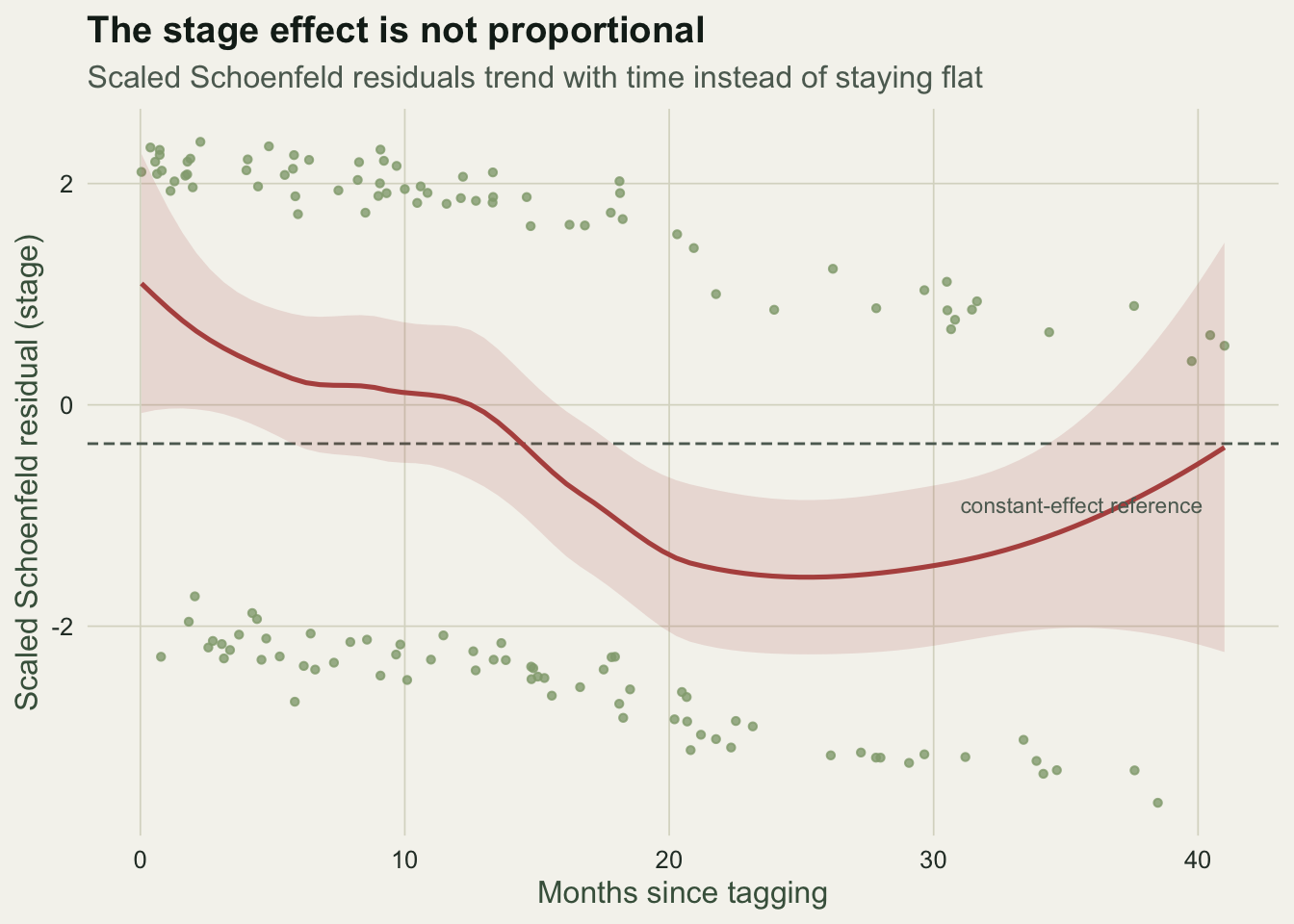

Figure 1: Scaled Schoenfeld residuals for stage against time; a flat scatter would support proportional hazards, but the smooth slopes clearly, so the stage effect changes with time.

The residuals drift from positive to negative across the follow-up: early on the juvenile hazard sits above the adult one, later it sits below. A single ratio cannot describe an effect that reverses, and reporting one would mislead about both the size and the direction of the stage difference at any particular age.

What the crossing looks like, and how to handle it

The mechanism is visible in the raw survival curves. Where proportional hazards hold, two Kaplan-Meier curves never cross; here they do, because the stage hazards swap order partway through.

kfit <- survfit(Surv(time, status) ~ stage, data = d)
grid <- seq(0, 42, by = 0.25)
kd <- lapply(levels(d$stage), function(g) {
  s <- summary(kfit[paste0("stage=", g)])
  data.frame(stage = g, time = grid, surv = stepfun(s$time, c(1, s$surv))(grid))
}) |> bind_rows()

ggplot(kd, aes(time, surv, colour = stage)) +
  geom_line(linewidth = 0.9) +
  scale_colour_manual(values = c(Adult = te_forest, Juvenile = te_gold)) +
  annotate("text", x = 40, y = 0.38, label = "Juvenile", colour = "#8a7a30", hjust = 1, size = 3.2) +
  annotate("text", x = 40, y = 0.11, label = "Adult", colour = te_forest, hjust = 1, size = 3.2) +
  coord_cartesian(ylim = c(0, 1)) +
  labs(title = "Crossing curves break proportional hazards",
       subtitle = "Juveniles die faster early, adults faster late",
       x = "Months since tagging", y = "Survival probability") +
  theme_te()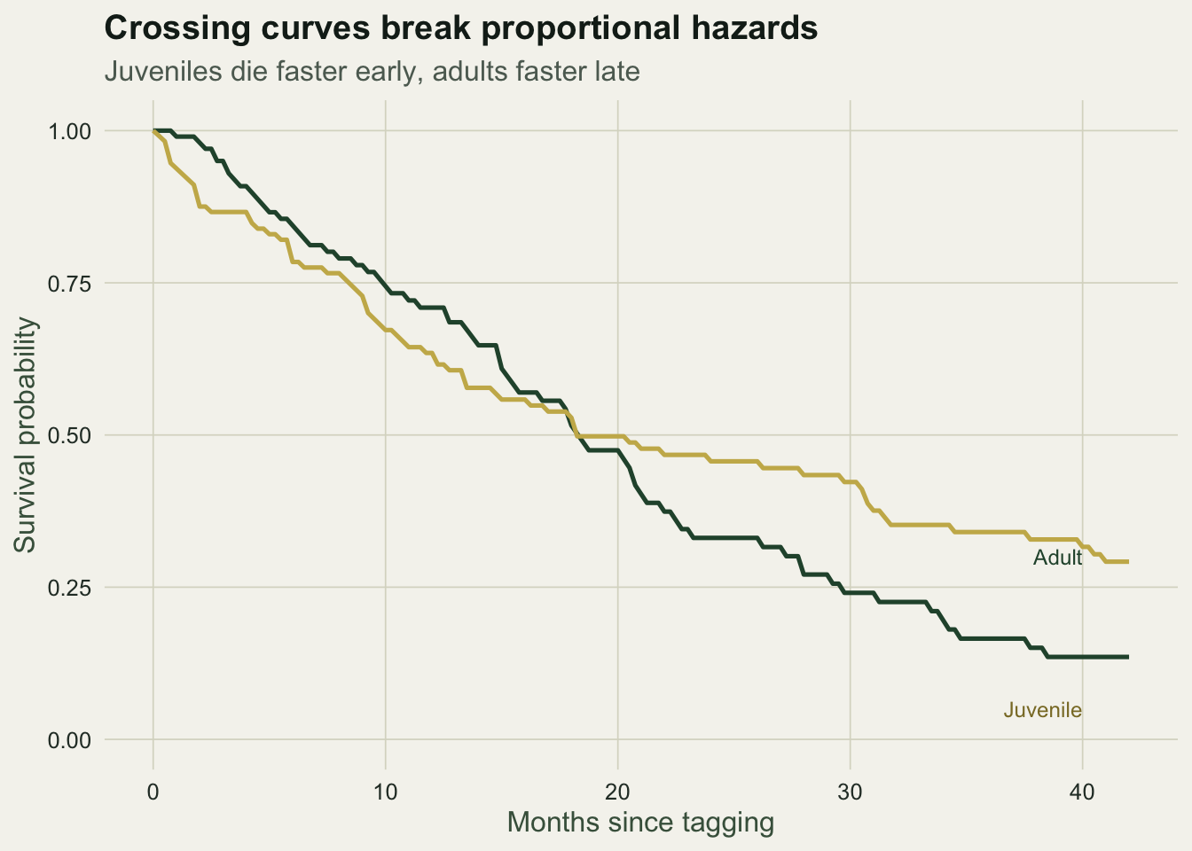

Figure 2: Kaplan-Meier curves by stage; the curves cross, the fingerprint of non-proportional hazards that a single ratio cannot capture.

The standard fix is to stratify by the offending covariate. Stratification lets each stage keep its own unspecified baseline hazard, so the model no longer forces a constant stage ratio, and estimates the parasite effect within strata.

m2 <- coxph(Surv(time, status) ~ parasite + strata(stage), data = d)
c(parasite_HR = round(exp(coef(m2)["parasite"]), 3),
  lower = round(exp(confint(m2)["parasite", 1]), 3),
  upper = round(exp(confint(m2)["parasite", 2]), 3))

parasite_HR.parasite                lower                upper 
               1.892                1.575                2.272 

cox.zph(m2)$table["GLOBAL", ]

     chisq         df          p 
3.23277738 1.00000000 0.07217818 

Inside the strata the parasite hazard ratio is 1.89, against 1.79 from the unstratified fit, and now free of contamination from the mis-modelled stage effect. Stratification removes the stage violation by construction rather than by passing a test: stage leaves the coefficient table, so the global test on the stratified model asks only about the parasite row, and that row can still fail it. Here it returns 0.072, which does not cross the usual threshold. Stage is no longer reported as a hazard ratio at all, which is honest: its effect was never a single number. When the changing effect itself is of interest, a time-by-covariate interaction estimates how the hazard ratio moves rather than hiding it.

Where to go next

The Cox model extends the survival analysis begun with Kaplan-Meier curves to covariates, and its assumption check is one instance of the wider habit of testing what a model takes for granted, the same discipline as residual diagnostics for a generalised linear model. When survival must be estimated from repeated captures instead of known fates, the Cormack-Jolly-Seber model plays the Cox role for detection-limited data, and when the response is whether a nest survives a monitoring interval, the logistic-exposure model carries covariates into daily survival.

References

Cox DR 1972. Journal of the Royal Statistical Society: Series B 34(2):187-202 (10.1111/j.2517-6161.1972.tb00899.x).

Schoenfeld D 1982. Biometrika 69(1):239-241 (10.1093/biomet/69.1.239).

Grambsch PM, Therneau TM 1994. Biometrika 81(3):515-526 (10.1093/biomet/81.3.515).

Therneau TM, Grambsch PM 2000. Modeling Survival Data: Extending the Cox Model. Springer. ISBN 978-0-387-98784-2.

Related tutorials

• Kaplan-Meier survival curves and the log-rank test
• Latency tests when some animals never respond
• Checking a survival model
• Time-varying covariates in a survival model

Reproducibility

• Code last run: 2026-09-30
• R version 4.5.3 (2026-03-11), aarch64-apple-darwin20
• Packages: dplyr 1.2.1, ggplot2 4.0.3, survival 3.8-12