library(ggplot2)
library(patchwork)
library(survival)

te_paper  <- "#f5f4ee"
te_ink    <- "#16241d"
te_body   <- "#2c3a31"
te_forest <- "#275139"
te_rust   <- "#b5534e"
te_gold   <- "#c9b458"
te_line   <- "#dad9ca"

theme_datasheet <- function() {
  theme_minimal(base_size = 12) +
    theme(plot.background  = element_rect(fill = te_paper, colour = NA),
          panel.background = element_rect(fill = te_paper, colour = NA),
          panel.grid.major = element_line(colour = te_line, linewidth = 0.3),
          panel.grid.minor = element_blank(),
          text             = element_text(colour = te_body),
          plot.title       = element_text(colour = te_ink, face = "bold"),
          plot.subtitle    = element_text(colour = te_body),
          axis.text        = element_text(colour = te_body))
}

n_animal    <- 600
tau_follow  <- 5
rate_change <- 0.4
haz_base    <- 0.35
hr_true     <- 1.0
n_rep <- 200Time-varying covariates in a survival model
R
survival analysis
causal inference
ecology tutorial
An ever infected label creates immortal time and a false protective hazard ratio. Coding time-varying covariates as start-stop rows in R with survival.
Corrected 25 September 2026: the honest limits said that coding a change seen only at visits biases the analysis in an unknown direction. The direction is known and is now measured in a separate post; the sentence says so.
A tagging study follows six hundred marked animals for five years. During those five years some of them acquire something: a chronic infection, a territory, a first successful brood, a rank in a dominance hierarchy. The field question is whether the animals that acquired it died faster or slower than the animals that never did.
The data arrive as one row per animal, and the obvious way to code the acquisition is a column that says whether it ever happened. That column is written once, at the end of the study, and it applies to the whole of the animal’s follow-up including the part that ran before the acquisition. It reads as a property the animal had all along.
It is not one. To be recorded as having changed state, an animal has to survive long enough to change state. The stretch of follow-up between time zero and the change is a stretch during which the animal could not have died, because if it had died it would have gone into the other group. Charging that stretch to the changed group hands it survival time in which no death was possible. The epidemiological name for it is immortal time, and Suissa 2008 lays out how it enters a drug study through exactly the same door.
This post simulates a cohort in which the state change has no effect on mortality at all, fits the naive coding, measures how large a protective effect it manufactures, and then fits the (start, stop] counting process coding that removes it. Two neighbouring posts sit close enough to be worth separating from this one immediately. Checking a survival model carries the Schoenfeld test, which asks whether an effect stays constant over time; this post asks whether a covariate’s value stays constant over time. Those are different failures with similar names, and one of them is measured below on the broken model here. Frailty and recurrent event models already uses the (start, stop] layout, in the Andersen-Gill section, where the reason is that one animal contributes several events. Same data layout, different reason for reaching for it.
An animal has to survive to the change to be counted as changed
Each animal has a time at which it changes state, drawn from an exponential distribution, and a death time generated from a hazard that is constant before the change and multiplied by the true hazard ratio after it. The true hazard ratio is set to one: the state change does nothing.
The cohort is 600 animals followed for 5 years. The generator inverts the cumulative hazard by hand rather than calling a package, because the piecewise shape is the whole point: the hazard is haz_base until the change and haz_base * hr after it.
sim_cohort <- function(n, hr) {
  t_change <- rexp(n, rate_change)
  u_draw   <- -log(runif(n))
  h_at_ch  <- haz_base * t_change
  t_death  <- ifelse(u_draw <= h_at_ch,
                     u_draw / haz_base,
                     t_change + (u_draw - h_at_ch) / (haz_base * hr))
  t_obs <- pmin(t_death, tau_follow)
  data.frame(id = seq_len(n), t_change = t_change, t_obs = t_obs,
             dead = as.integer(t_death <= tau_follow),
             ever = as.integer(t_change < t_obs))
}

set.seed(20260809)
cohort <- sim_cohort(n_animal, hr_true)

n_dead <- sum(cohort$dead); n_ever <- sum(cohort$ever)
imm_time  <- sum(cohort$t_change[cohort$ever == 1])
time_ever <- sum(cohort$t_obs[cohort$ever == 1]); time_all <- sum(cohort$t_obs)
imm_share <- 100 * imm_time / time_ever; imm_all <- 100 * imm_time / time_all
mean_ever <- mean(cohort$t_obs[cohort$ever == 1])
mean_none <- mean(cohort$t_obs[cohort$ever == 0])
died_ever <- 100 * mean(cohort$dead[cohort$ever == 1])
died_none <- 100 * mean(cohort$dead[cohort$ever == 0])
501 of the 600 animals died inside the five years, and 342 changed state before they left the study. Those 342 animals contribute 1080 animal years of follow-up, of which 418 years, 39 per cent, ran before the change. Across the whole cohort that immortal stretch is 30 per cent of all the follow-up in the study.
Zero deaths occurred in it, and not because the state change was protective. It is arithmetic: a death before the change would have put the animal in the never changed group. The naive column hands the changed group a large block of guaranteed survival and then asks a model to compare death rates.
The symptom is visible before any model runs. Animals labelled as changed were followed for 3.16 years on average against 1.27 years for the rest, and 74 per cent of them died against 96 per cent. Nothing about the change caused any of that.
The same risk-set error wears a different costume in nest survival with logistic exposure, where nests found part way through the cycle only had to survive the days that remained. There the misattributed time sits at the start of the observation rather than at the start of the covariate, but the accounting mistake is identical: credit for survival that was never at risk of being contradicted.
show_ever <- head(cohort$id[cohort$ever == 1], 7)
show_none <- head(cohort$id[cohort$ever == 0], 7)
tl <- cohort[cohort$id %in% c(show_none, show_ever), ]
tl$rowpos <- match(tl$id, c(show_none, show_ever))

tl_ever <- tl[tl$ever == 1, ]
tl_none <- tl[tl$ever == 0, ]
seg_all <- rbind(
  data.frame(y = tl_none$rowpos, x0 = 0, x1 = tl_none$t_obs, part = "never changed"),
  data.frame(y = tl_ever$rowpos, x0 = 0, x1 = tl_ever$t_change, part = "before the change"),
  data.frame(y = tl_ever$rowpos, x0 = tl_ever$t_change, x1 = tl_ever$t_obs,
             part = "after the change"))
seg_all$part <- factor(seg_all$part,
                       levels = c("never changed", "before the change", "after the change"))

ggplot(seg_all) +
  geom_segment(aes(x = x0, xend = x1, y = y, yend = y, colour = part),
               linewidth = 2.1, lineend = "butt") +
  geom_point(data = tl_ever, aes(t_change, rowpos), shape = 21, size = 2.6,
             stroke = 0.9, colour = te_ink, fill = te_paper) +
  geom_point(data = tl[tl$dead == 1, ], aes(t_obs, rowpos), size = 2.4,
             colour = te_rust) +
  scale_colour_manual(values = c("never changed" = te_line,
                                 "before the change" = te_gold,
                                 "after the change" = te_forest), name = NULL) +
  scale_x_continuous(limits = c(0, tau_follow + 0.15), expand = c(0.01, 0)) +
  scale_y_continuous(breaks = NULL) +
  labs(x = "years since marking", y = NULL,
       title = "The gold stretch is immortal time",
       subtitle = "open circle: state change; red dot: death") +
  theme_datasheet() +
  theme(legend.position = "bottom")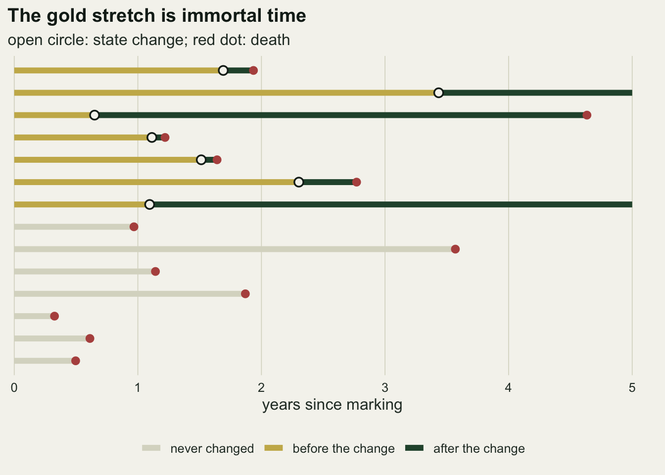
The naive coding manufactures a protective effect
One column, one model, and the answer is emphatic and wrong.
fit_naive <- coxph(Surv(t_obs, dead) ~ ever, data = cohort)

hr_naive <- unname(exp(coef(fit_naive)))
ci_naive <- unname(exp(confint(fit_naive)))
p_naive <- summary(fit_naive)$coefficients[1, 5]; pct_drop <- 100 * (1 - hr_naive)
The fitted hazard ratio is 0.283, with a 95 per cent interval of 0.236 to 0.340, against a truth of 1.0. Read as biology it says the state change cuts the risk of death by 72 per cent, at a p value of \(6.8 \times 10^{-42}\). The interval does not come close to containing one, so no amount of caution about statistical significance would have saved the conclusion. The effect is large, tight and entirely an artefact of the coding.
The counting process coding removes it
The repair is to stop pretending the covariate had one value for the whole of follow-up. Every animal that changed state is split into two rows: an interval from zero to the change with the covariate at zero, and an interval from the change to the exit with the covariate at one. Animals that never changed keep a single row. The event indicator belongs to the row that contains the exit, so the first row of a split animal is censored at the change.
to_counting <- function(d) {
  ch <- d$t_change < d$t_obs
  pre <- data.frame(id = d$id, t0 = 0,
                    t1 = ifelse(ch, d$t_change, d$t_obs),
                    event = ifelse(ch, 0L, d$dead), state = 0L)
  post <- data.frame(id = d$id[ch], t0 = d$t_change[ch], t1 = d$t_obs[ch],
                     event = d$dead[ch], state = 1L)
  rbind(pre, post)
}

cp <- to_counting(cohort)
fit_td <- coxph(Surv(t0, t1, event) ~ state, data = cp)

hr_td   <- unname(exp(coef(fit_td)))
ci_td   <- unname(exp(confint(fit_td)))
n_rows <- nrow(cp); ev_cp <- sum(cp$event)
ev_pre <- sum(cp$event[cp$state == 0]); ev_post <- sum(cp$event[cp$state == 1])
600 animals become 942 rows carrying the same 501 deaths, 247 of them while the covariate was still zero and 254 after it turned to one. The deaths did not move; only the exposure they are compared against did. The hazard ratio is now 1.180, with an interval of 0.962 to 1.448, which contains one. The point estimate sits above one in this particular cohort, which is sampling noise rather than a residual bias; the replicate study below shows how wide that scatter is.
This estimate is noisier than the naive one, and that is the correct direction. The naive standard error was small because the comparison it was making, between animals that survived a long time and animals that did not, is a comparison the data can make very sharply. It was the wrong comparison. Andersen & Gill 1982 gave the counting process formulation the large sample theory that lets coxph treat these split rows as legitimate; Therneau & Grambsch 2000 is the practical treatment, and the tmerge function in the same package builds the split for real data with several time-varying columns instead of the two-row case written out by hand here.
One line in the split deserves attention. t0 for the second row is the change time, not zero. Dropping that column and fitting Surv(t1, event) ~ state would put every post-change interval back into the risk set from time zero and rebuild the bias in a different disguise.
km <- survfit(Surv(t_obs, dead) ~ ever, data = cohort)
km_df <- rbind(
  data.frame(time = 0, surv = 1, grp = c("never changed", "ever changed")),
  data.frame(time = km$time, surv = km$surv,
             grp = rep(c("never changed", "ever changed"), km$strata)))

p_km <- ggplot(km_df, aes(time, surv, colour = grp)) +
  geom_step(linewidth = 1) +
  annotate("text", x = 3.4, y = 0.72, label = "ever changed", colour = te_gold,
           hjust = 0, size = 3.4) +
  annotate("text", x = 1.9, y = 0.30, label = "never changed", colour = te_body,
           hjust = 0, size = 3.4) +
  scale_colour_manual(values = c("never changed" = te_body,
                                 "ever changed" = te_gold),
                      guide = "none") +
  scale_y_continuous(limits = c(0, 1)) +
  scale_x_continuous(limits = c(0, tau_follow)) +
  labs(x = "years", y = "surviving fraction",
       title = "Split by the naive label",
       subtitle = "a gap from an effect of nothing") +
  theme_datasheet()

lab_naive <- "naive:\never changed"
lab_td    <- "time-dependent:\n(start, stop]"
est_df <- data.frame(
  method = factor(c(lab_naive, lab_td), levels = c(lab_td, lab_naive)),
  est = c(hr_naive, hr_td),
  lo  = c(ci_naive[1], ci_td[1]),
  hi  = c(ci_naive[2], ci_td[2]))

p_est <- ggplot(est_df, aes(est, method)) +
  geom_vline(xintercept = hr_true, colour = te_rust,
             linetype = "dashed", linewidth = 0.8) +
  geom_errorbar(aes(xmin = lo, xmax = hi), orientation = "y", width = 0.14,
                colour = te_forest, linewidth = 0.7) +
  geom_point(size = 3, colour = te_forest) +
  scale_x_log10(breaks = c(0.25, 0.5, 1, 1.5), limits = c(0.2, 1.9)) +
  labs(x = "hazard ratio (log scale)", y = NULL,
       title = "Two codings",
       subtitle = "dashed red: the truth") +
  theme_datasheet()

p_km + p_est + plot_layout(widths = c(1.15, 1)) +
  plot_annotation(theme = theme_datasheet())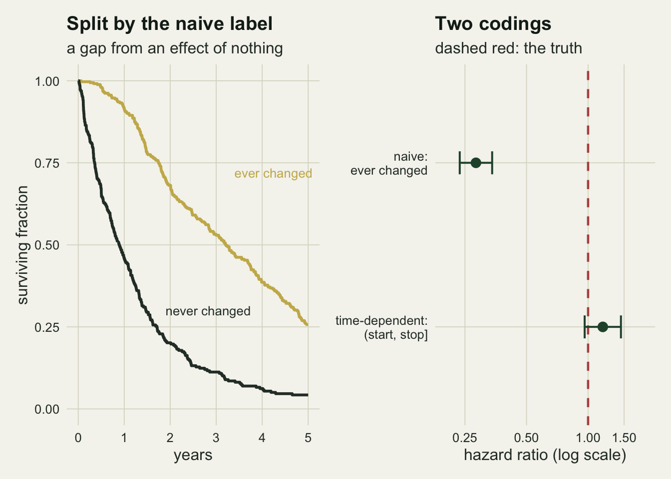
The proportional hazards test fires, and points at the wrong repair
A reader who fits the naive model and then follows the usual checking routine will run cox.zph on it. The test is worth running on the broken fit, and so are the repairs it invites, because not one of them does what a reader would expect.
zph_naive <- cox.zph(fit_naive)
zph_chisq <- unname(zph_naive$table[1, 1])
zph_p     <- unname(zph_naive$table[1, 3])
zph_cor   <- unname(cor(zph_naive$y[, 1], zph_naive$x))

brk_lo <- 1; brk_hi <- 2
split_dat <- survSplit(Surv(t_obs, dead) ~ ., data = cohort,
                       cut = c(brk_lo, brk_hi), episode = "period")
fit_strat <- coxph(Surv(tstart, t_obs, dead) ~ ever + strata(period), data = split_dat)
b_naive <- unname(coef(fit_naive)); b_strat <- unname(coef(fit_strat))
hr_strat <- exp(b_strat); b_gap <- abs(b_strat - b_naive); n_split <- nrow(split_dat)

fit_period <- coxph(Surv(tstart, t_obs, dead) ~ ever:factor(period) + strata(period),
                    data = split_dat)
hr_period <- unname(exp(coef(fit_period)))

fit_within <- coxph(Surv(t_obs, dead) ~ strata(ever), data = cohort)
n_coef_ever <- length(coef(fit_within))

fit_tt <- coxph(Surv(t_obs, dead) ~ ever + tt(ever), data = cohort,
                tt = function(x, tm, ...) x * tm)
hr_tt0 <- unname(exp(coef(fit_tt)[1])); b_tt_time <- unname(coef(fit_tt)[2])
The Schoenfeld test rejects hard: a chi-squared of 42.0 on one degree of freedom, p equal to \(9.2 \times 10^{-11}\). It has noticed something real. The correlation between the scaled Schoenfeld residuals and the transformed time axis cox.zph uses is +0.306, and a separate coefficient fitted in each of three periods of follow-up, split at 1 and 2 years, gives hazard ratios of 0.109, 0.348 and 0.520. The apparent protection is strongest early, when the immortal stretches are long relative to the follow-up so far, and it fades later. The fitted effect really does drift with time.
The trouble is what the test invites next. The standard responses to a rejected proportional hazards assumption are to stratify follow-up into periods, to stratify on the offending variable, or to let its coefficient vary with time. All of them keep the covariate as it was coded.
The first does nothing whatsoever. Splitting every animal’s follow-up at those two points with survSplit, which turns 600 rows into 1316, and then fitting ever + strata(period), returns a log hazard ratio of -1.262460 against the naive model’s -1.262460. The two are equal to within floating point rounding. The hazard ratio is still 0.283.
That is exact, not approximate. A Cox partial likelihood is already local in time: each death is compared only with the animals at risk at that instant, and every one of them sits in the same period the death does. Cutting time into periods and stratifying on period sorts the same comparisons into the same groups and multiplies the same terms together. Splitting can only change an estimate when something in the model differs across the pieces: a covariate whose value moves, or a coefficient allowed to differ by period. Here ever does neither, because it was written once, at the end of the study.
The second response empties the model. Stratifying on ever gives the changed and the unchanged animals separate baseline hazards and compares each animal only inside its own group, which leaves 0 coefficients to report. The bias is gone because the comparison is gone, and the question the study asked went with it.
The third response does move the estimate. A tt(ever) term, the covariate multiplied by time, puts the hazard ratio at 0.107 at the time origin with a time coefficient of +0.568, so the fitted protection weakens as follow-up runs on, which is what the period fits above already said. Every one of those period estimates is far below the true 1.0, and so is the value at the origin. The time interaction describes the fade accurately and still reports a large protective effect through most of a study in which the state change does nothing, the fitted ratio climbing past one only near the end of the follow-up.
The three responses fail for one reason. The proportional hazards test is right that the effect is not constant, and no repair aimed at the shape of the hazard reaches this bias, because the bias is not in the shape. It is in the definition of the covariate, a value fixed by the animal’s future. The proportional hazards assumption is about whether an effect stays constant; this failure is about whether a covariate’s value stays constant. The names are close and the fixes do not overlap. In practice that makes the order matter: run the time-dependent coding first, then check proportional hazards on the model that has the covariate right, because a proportional hazards test on a mis-coded covariate is testing the wrong thing carefully.
Landmarking gets the same answer from fewer animals
The counting process coding needs the change time. Field data often gives only the state at each visit, so the exact time is unknown. The cheap alternative is a landmark analysis, introduced for exactly this problem by Anderson, Cain & Gelber 1983: pick a landmark time, discard every animal that left the study before it, classify the survivors by the state they were in at the landmark, and analyse survival from the landmark onwards. No animal can then be classified using information from after the clock starts.
fit_at_landmark <- function(d, lmk) {
  kept <- d[d$t_obs > lmk, ]
  kept$state_lmk <- as.integer(kept$t_change <= lmk)
  fit <- coxph(Surv(t_obs - lmk, dead) ~ state_lmk, data = kept)
  c(hr = unname(exp(coef(fit))), lo = unname(exp(confint(fit)))[1],
    hi = unname(exp(confint(fit)))[2], n_kept = nrow(kept),
    n_ev = sum(kept$dead))
}

lmk_main <- 1.5
lm_one   <- fit_at_landmark(cohort, lmk_main)
lmk_grid <- seq(0.25, 3, by = 0.25)
lm_sweep <- as.data.frame(t(vapply(lmk_grid, function(z)
  fit_at_landmark(cohort, z), numeric(5))))
lm_sweep$lmk <- lmk_grid

kept_pct  <- 100 * lm_one[["n_kept"]] / n_animal
lost_n    <- n_animal - lm_one[["n_kept"]]
n_exclude <- sum(lm_sweep$lo > hr_true | lm_sweep$hi < hr_true)
n_sweep   <- nrow(lm_sweep)
conf_pct  <- 95
exp_miss  <- n_sweep * (1 - conf_pct / 100)
p_miss    <- binom.test(n_exclude, n_sweep, 1 - conf_pct / 100)$p.value
A landmark at 1.5 years keeps 342 of the 600 animals, 57 per cent, and returns a hazard ratio of 1.005 with an interval of 0.781 to 1.293. The bias is gone. The 258 animals that died before the landmark are gone with it, and so is every state change that happened after it: an animal that changes at year four is analysed as though it never changed.
p_hr <- ggplot(lm_sweep, aes(lmk, hr)) +
  geom_hline(yintercept = hr_true, colour = te_rust,
             linetype = "dashed", linewidth = 0.8) +
  geom_errorbar(aes(ymin = lo, ymax = hi), width = 0.07,
                colour = te_forest, linewidth = 0.5) +
  geom_point(size = 2.4, colour = te_forest) +
  scale_x_continuous(limits = c(0.1, 3.15)) +
  labs(x = NULL, y = "hazard ratio",
       title = "The bias is gone at every landmark",
       subtitle = "dashed red: the true hazard ratio") +
  theme_datasheet() +
  theme(axis.text.x = element_blank())

size_df <- data.frame(
  lmk = rep(lmk_grid, 2),
  n   = c(lm_sweep$n_kept, lm_sweep$n_ev),
  what = rep(c("animals retained", "deaths retained"), each = n_sweep))

p_n <- ggplot(size_df, aes(lmk, n, colour = what)) +
  geom_line(linewidth = 0.9) +
  geom_point(size = 2) +
  scale_colour_manual(values = c("animals retained" = te_ink,
                                 "deaths retained" = te_gold), name = NULL) +
  scale_y_continuous(limits = c(0, NA)) +
  scale_x_continuous(limits = c(0.1, 3.15)) +
  labs(x = "landmark time (years)", y = "count",
       title = "What each landmark costs") +
  theme_datasheet() +
  theme(legend.position = "bottom")

p_hr / p_n + plot_annotation(theme = theme_datasheet())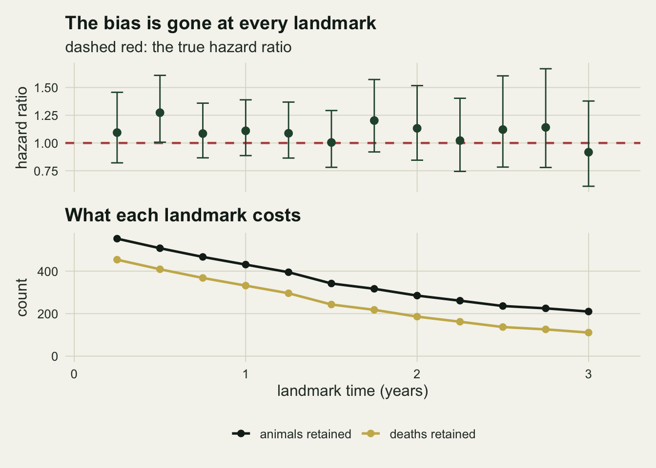
The sweep carries a warning of its own, though not the one the eye reaches for first. 1 of the 12 intervals excludes the truth, against the 0.6 misses that 12 intervals at 95 per cent coverage should produce on average; testing that count against the nominal miss rate gives p equal to 0.46. The fits are nested subsets of one cohort as well, so they are heavily correlated and are not independent trials in any case. The problem is not that a landmark missed. It is that the analyst can see which one did, and a landmark chosen after looking at the answer is a researcher degree of freedom with real teeth. Pick the landmark from the biology, before the analysis: the age at which a state change becomes possible, or the first visit at which every animal has been assessed.
Two hundred replicates put numbers on all three
One cohort is one draw. The same generator run 200 times, with the same true hazard ratio of one, gives the median estimate and the rejection rate of each coding.
one_replicate <- function(lmk) {
  d  <- sim_cohort(n_animal, hr_true)
  fn <- coxph(Surv(t_obs, dead) ~ ever, data = d)
  ft <- coxph(Surv(t0, t1, event) ~ state, data = to_counting(d))
  kept <- d[d$t_obs > lmk, ]
  kept$state_lmk <- as.integer(kept$t_change <= lmk)
  fl <- coxph(Surv(t_obs - lmk, dead) ~ state_lmk, data = kept)
  c(b_n = unname(coef(fn)), s_n = sqrt(vcov(fn))[1],
    b_t = unname(coef(ft)), s_t = sqrt(vcov(ft))[1],
    b_l = unname(coef(fl)), s_l = sqrt(vcov(fl))[1],
    n_l = nrow(kept))
}

set.seed(4471)
reps <- as.data.frame(t(replicate(n_rep, one_replicate(lmk_main))))

n_reject <- function(b, s) sum(abs(b / s) > 1.96)
wilson_pct <- function(k, n, z = 1.96) {
  ph  <- k / n
  mid <- (ph + z^2 / (2 * n)) / (1 + z^2 / n)
  hw  <- z * sqrt(ph * (1 - ph) / n + z^2 / (4 * n^2)) / (1 + z^2 / n)
  100 * c(max(0, mid - hw), min(1, mid + hw))
}

med_n <- exp(median(reps$b_n)); k_n <- n_reject(reps$b_n, reps$s_n)
med_t <- exp(median(reps$b_t)); k_t <- n_reject(reps$b_t, reps$s_t)
med_l <- exp(median(reps$b_l)); k_l <- n_reject(reps$b_l, reps$s_l)
rej_n <- 100 * k_n / n_rep; rej_t <- 100 * k_t / n_rep; rej_l <- 100 * k_l / n_rep
ci_rej_t <- wilson_pct(k_t, n_rep); ci_rej_l <- wilson_pct(k_l, n_rep)
se_cost <- mean(reps$s_l) / mean(reps$s_t); kept_avg <- 100 * mean(reps$n_l) / n_animal
nominal  <- 5
The naive coding has a median hazard ratio of 0.301 and rejects the true null in 100 per cent of the 200 replicates. Not 5 per cent: every single replicate declared a protective effect that does not exist. This is not a test with poor power or an inflated error rate that careful reading would catch. The quantity it estimates is not the hazard ratio, and at this cohort size it sits far enough from one, relative to its standard error, that the test rejects in every replicate run here.
The time-dependent coding has a median of 0.987 and rejects 5 times out of 200, which is 2.5 per cent with a Wilson interval of 1.1 to 5.7 per cent: the nominal 5 per cent is inside it. The landmark analysis has a median of 0.982, rejects 14 times, 7.0 per cent with an interval of 4.2 to 11.4 per cent, which also covers the nominal level. It pays for that with standard errors 1.22 times wider than the time-dependent fit while keeping 59 per cent of the cohort on average.
coding_lab <- c("naive: ever changed", "time-dependent: (start, stop]",
                sprintf("landmark at %.1f years", lmk_main))
rep_long <- data.frame(
  hr = exp(c(reps$b_n, reps$b_t, reps$b_l)),
  coding = factor(rep(coding_lab, each = n_rep), levels = coding_lab))

ggplot(rep_long, aes(hr)) +
  geom_histogram(bins = 34, fill = te_forest, colour = te_paper, linewidth = 0.2) +
  geom_vline(xintercept = hr_true, colour = te_rust,
             linetype = "dashed", linewidth = 0.8) +
  facet_wrap(~ coding, ncol = 1) +
  scale_x_log10(breaks = c(0.25, 0.5, 0.75, 1, 1.5)) +
  labs(x = "estimated hazard ratio (log scale)", y = "replicates",
       title = "The same truth, read three ways",
       subtitle = "dashed red: the true hazard ratio") +
  theme_datasheet() +
  theme(strip.text = element_text(colour = te_ink))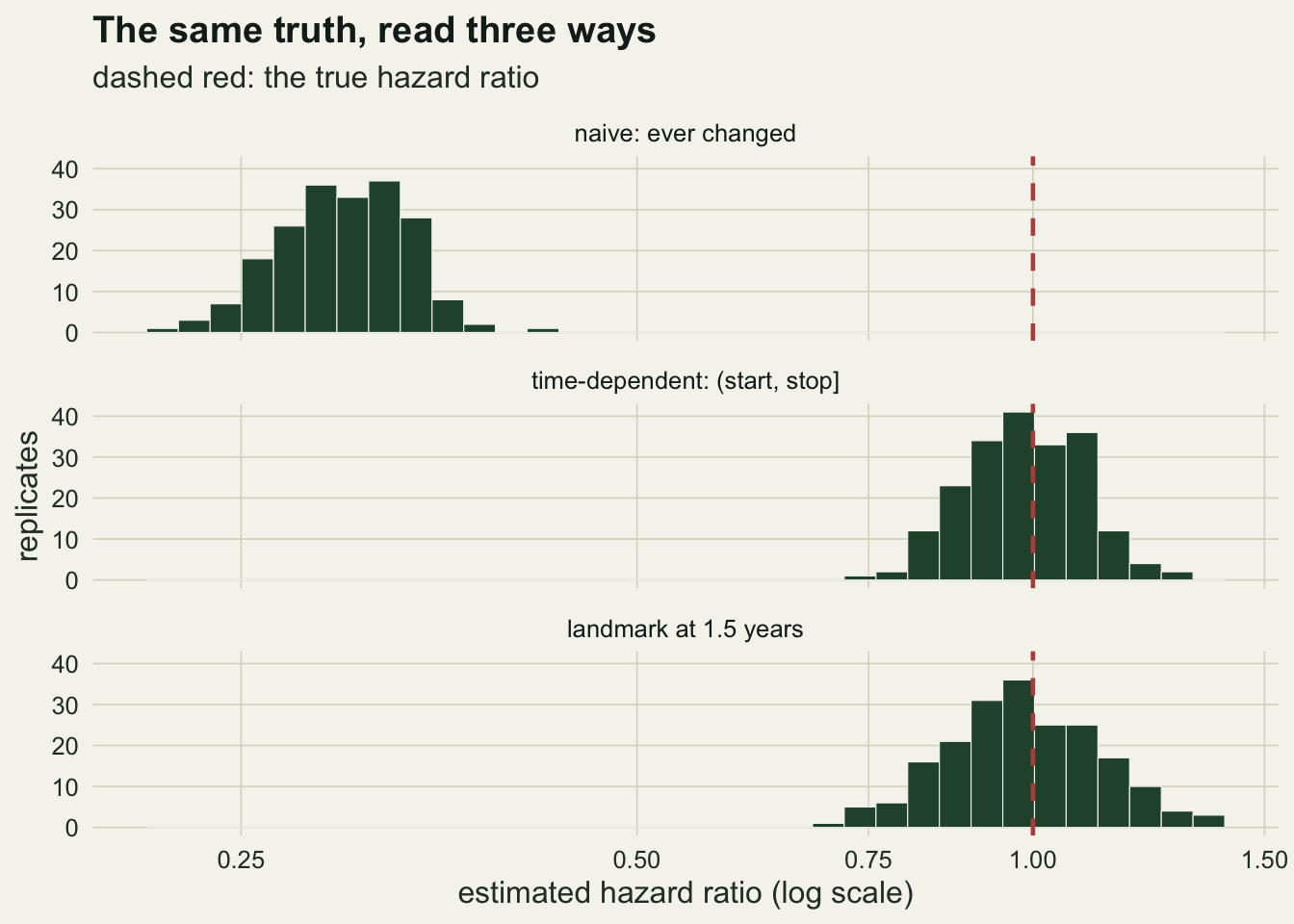
What to report
State when the covariate was measured relative to the time origin. A survival analysis with a covariate that was recorded after follow-up began is a different analysis from one whose covariates were all fixed at marking, and a reader cannot tell which they are looking at from a coefficient table.
If the change time is known, say that the model used start and stop intervals, and give the number of rows and the number of animals separately. Those two counts differ, and a table that reports only rows invites a reader to think the sample is larger than it is.
Give the number of animals that changed state and the distribution of the change times. A covariate that switches on late for most animals carries little information about the post-change hazard, however many animals eventually switch, and the interval will show it.
If a landmark analysis was used instead, give the landmark, how it was chosen, how many animals were excluded for leaving before it, and how many changed state after it and were therefore analysed in the wrong state. State that the estimate applies to animals that survived to the landmark, because it does.
Report the choice of time origin. Fieberg & DelGiudice 2009 works through what changes when the clock starts at capture rather than at birth or at a calendar date, and the choice interacts with a time-varying covariate: a covariate that switches at a fixed age is a different variable when time runs from capture.
Honest limits
The time-dependent coding assumes the change time is known. If the state is only observed at visits, all that is known is that the change happened somewhere between two of them, and that is interval censoring, which is a different problem this post does not solve. Putting the change at the midpoint of the interval pushes the hazard ratio towards protection even when the state does nothing, and coding it at the visit that detected it shrinks a real effect towards one; a state change seen only at visits measures both and fits the illness-death likelihood that repairs them. Fieberg & DelGiudice 2008 treats the interval-censored case properly for wildlife monitoring data, and the landmark analysis above is the cheap version of the same retreat.
The simulation makes the state change independent of everything else. In a real study the animals that acquire an infection or a territory are usually not a random subset: they are the bolder ones, the older ones, the ones in better condition. The counting process coding removes the immortal time; it does not remove confounding by whatever else predicts both the change and the death. Nothing in the split rows knows that the two groups differ before the change.
The change here is one way and permanent. Covariates that switch back and forth, or continuous covariates that are remeasured at each visit, need more rows and one more assumption: that the value recorded at a visit holds until the next one. That step function is a modelling choice and it is rarely stated as one.
The state change is also assumed not to be a consequence of impending death. If animals shed a territory or lose condition in their final weeks, the covariate is partly a marker of the death that is about to happen, and the time-dependent estimate absorbs that as an effect. No coding fixes a covariate that is downstream of the outcome; only a design that measures the covariate before the process that kills the animal does.
The replicate study uses 200 replicates, which pins a rejection rate near the nominal level down only to a few percentage points: the interval for the landmark analysis runs from 4.2 to 11.4 per cent, so whether it is exactly nominal or slightly above it is not settled here. Separating 100 per cent from 5 per cent needs no such care, and the finding that survives is about the naive coding. A true hazard ratio of exactly one was chosen for the same reason, so that everything the naive model reports is bias; with a real effect the bias does not disappear but adds to the effect on the log scale, and a state change that genuinely raises mortality can then be reported as protective, as neutral, or as harmful but understated, depending on how much immortal time the design happens to create.
References
Andersen PK, Gill RD 1982 Annals of Statistics 10:1100-1120 (10.1214/aos/1176345976)
Anderson JR, Cain KC, Gelber RD 1983 Journal of Clinical Oncology 1(11):710-719 (10.1200/JCO.1983.1.11.710)
Fieberg J, DelGiudice GD 2008 Journal of Wildlife Management 72(5):1211-1219 (10.2193/2007-403)
Fieberg J, DelGiudice GD 2009 Ecology 90(6):1687-1697 (10.1890/08-0724.1)
Suissa S 2008 American Journal of Epidemiology 167(4):492-499 (10.1093/aje/kwm324)
Therneau TM, Grambsch PM 2000 Modeling Survival Data: Extending the Cox Model. Springer. ISBN 978-0-387-98784-2