library(ggplot2)
library(patchwork)
library(survival)

te_paper  <- "#f5f4ee"
te_ink    <- "#16241d"
te_body   <- "#2c3a31"
te_forest <- "#275139"
te_rust   <- "#b5534e"
te_gold   <- "#c9b458"
te_line   <- "#dad9ca"

theme_datasheet <- function() {
  theme_minimal(base_size = 12) +
    theme(plot.background  = element_rect(fill = te_paper, colour = NA),
          panel.background = element_rect(fill = te_paper, colour = NA),
          panel.grid.major = element_line(colour = te_line, linewidth = 0.3),
          panel.grid.minor = element_blank(),
          text             = element_text(colour = te_body),
          plot.title       = element_text(colour = te_ink, face = "bold"),
          plot.subtitle    = element_text(colour = te_body),
          axis.text        = element_text(colour = te_body))
}

n_animal    <- 300    # collared animals, all uninfected at marking
rate_change <- 0.4    # infections per animal-year
haz_base    <- 0.3    # deaths per animal-year before infection
tau_follow <- 4 # years of follow-upA state change seen only at visits
R
survival analysis
censoring
disease ecology
maximum likelihood
simulation
ecology tutorial
A state seen only at visits: an illness-death fit in R recovers the hazard ratio that midpoint coding pulls towards protection and the detection visit shrinks.
A population of badgers is trapped once a year. Every animal caught gets a blood test for a chronic infection and a collar with a mortality sensor, so the day each animal dies is known exactly from the collar, while its infection status is known only on the days it is caught. The question is whether infected animals die faster. An animal that tested negative at one trapping and positive at the next became infected somewhere in the year between, and the date is not in the data.
The post on time-varying covariates in a survival model builds the (start, stop] coding that removes immortal time when the change time is known, and its honest limits stop exactly here: “If the state is only observed at visits, all that is known is that the change happened somewhere between two of them, and that is interval censoring, which is a different problem this post does not solve.” It adds that putting the change at the midpoint of the interval, or at the visit that detected it, “biases the change time in a known direction and the analysis in an unknown one”. Its landmark section is the retreat that avoids the problem by classifying animals at one fixed time. This post takes the problem on: it measures the two reflex codings against a likelihood that uses only what the visits saw, and it shows that the direction of the midpoint’s bias is not unknown.
The comparison of the codings is published. Goggins, Finkelstein & Zaslavsky 1999 set out the problem, a binary time-varying covariate whose change time is interval censored in a Cox model, and repaired it by imputing the change times with a Monte Carlo EM algorithm. Nevo and colleagues (2020) compared last value carried forward, which is the detection-visit coding here, with midpoint imputation, and wrote that “In terminal main event scenarios, MidI had a very large bias, even under the null.” Their repair is a family of calibration models for the distribution of the change time. The repair used below is a third published one: an illness-death model, a three-state Markov process from healthy to changed to dead, fitted to states seen at visits and exact death times. Joly and colleagues (2002) fitted it with smooth intensities to dementia and death, and Leffondre and colleagues (2013) compared it with Cox regression for the effect of an exposure on an interval-censored illness when death competes, and concluded that it should be preferred when follow-up intervals are wide and the exposure affects mortality. So none of the results below is new. What the post adds is the likelihood written out in base R, a check of it over replicates on a wildlife design, the midpoint’s bias derived as person-time arithmetic, and a measurement of what the simple version of the repair does when mortality changes with time since marking.
Two other posts sit close. Interval-censored survival from visit data puts the death time, not a covariate’s change time, at the midpoint of a visit interval, and its own limits say “No covariates were fitted.” Multi-state capture-recapture fits a state process at discrete occasions with a forward likelihood, which is the capture-recapture relative of the likelihood here; there, death is never seen and detection is imperfect, while here death is timed exactly and every live visit happens.
Infection seen at yearly visits, death timed by the collar
Each animal is uninfected at marking and becomes infected at a constant rate of 0.4 a year. Before infection it dies at 0.3 a year, and after infection at 0.3 times the true hazard ratio. Follow-up lasts four years. The animal is visited at fixed intervals after marking for as long as it is alive, including a last visit at four years, and the test at each visit is perfect. Death is timed exactly, but the carcass is not tested: the infection state at death is known only through the visits before it. That is the field case simulated throughout, and it matters, because a necropsy that found the state at death would change the likelihood (the limits come back to it).
The generator inverts the cumulative hazard by hand, as in the source post. The shape argument, used only in the last section, lets the baseline hazard rise with time since marking.
sim_panel <- function(n, hr, dv, shape = 1) {
  t_change <- rexp(n, rate_change)
  u_draw   <- rexp(n)
  h_at     <- haz_base * t_change^shape          # cumulative hazard at the change
  t_death  <- ifelse(u_draw <= h_at, (u_draw / haz_base)^(1 / shape),
                     ((u_draw - h_at) / (haz_base * hr) + t_change^shape)^(1 / shape))
  t_obs <- pmin(t_death, tau_follow)
  dead  <- as.integer(t_death <= tau_follow)
  k_max <- round(tau_follow / dv)
  n_vis <- ifelse(dead == 1, pmin(floor(t_obs / dv), k_max), k_max)  # live visits after marking
  j_pos <- ceiling(t_change / dv)                                      # first visit after the change
  seen  <- j_pos <= n_vis
  t_detect <- ifelse(seen, j_pos * dv, Inf)
  data.frame(id = seq_len(n), t_change, t_obs, dead, n_vis, seen, t_detect,
             t_mid = ifelse(seen, t_detect - dv / 2, Inf))
}

hr_demo <- 3; dv_demo <- 1
set.seed(20261010)
cohort <- sim_panel(n_animal, hr_demo, dv_demo)

n_dead    <- sum(cohort$dead)
n_changed <- sum(cohort$t_change < cohort$t_obs)
n_seen    <- sum(cohort$seen)
n_unseen  <- sum(cohort$t_change < cohort$t_obs & !cohort$seen)
n_unseen_dead <- sum(cohort$t_change < cohort$t_obs & !cohort$seen & cohort$dead == 1)
n_seen_last   <- sum(cohort$seen & cohort$t_detect == cohort$t_obs)
In one cohort with a true hazard ratio of 3 and yearly visits, 254 of the 300 animals die within the four years and 152 become infected before they die or leave the study. The visits see 109 of those infections, 6 of them only at the final visit. The other 43 are never seen, and every one of those animals died before the next visit could find it infected; in this design no other way of being missed exists, because an animal alive at four years gets a last visit. Those deaths are the detection-visit coding’s problem. The midpoint coding has a different one, drawn in gold below.
pick <- c(head(cohort$id[cohort$seen & cohort$dead == 1 & cohort$t_detect < cohort$t_obs], 4),
          head(cohort$id[!cohort$seen & cohort$t_change < cohort$t_obs & cohort$dead == 1], 4),
          head(cohort$id[cohort$t_change >= cohort$t_obs & cohort$dead == 1], 2),
          head(cohort$id[cohort$t_change >= cohort$t_obs & cohort$dead == 0], 2))
tl <- cohort[match(pick, cohort$id), ]
tl$row <- rev(seq_along(pick))
grp_at <- c(10.5, 6.5, 2.5)
grp_lab <- c("seen infected", "infected,\ndied unseen", "never infected")
seg <- rbind(
  data.frame(row = tl$row, x0 = 0, x1 = pmin(tl$t_change, tl$t_obs), part = "uninfected"),
  data.frame(row = tl$row, x0 = pmin(tl$t_change, tl$t_obs), x1 = tl$t_obs, part = "infected"))
seg$part <- factor(seg$part, levels = c("uninfected", "infected"))
vis <- do.call(rbind, lapply(seq_len(nrow(tl)), function(i)
  if (tl$n_vis[i] > 0) data.frame(row = tl$row[i], x = seq_len(tl$n_vis[i]) * dv_demo,
                                  pos = seq_len(tl$n_vis[i]) * dv_demo >= tl$t_change[i])))
imm <- tl[tl$seen, ]

ggplot() +
  geom_segment(data = seg, aes(x = x0, xend = x1, y = row, yend = row, colour = part),
               linewidth = 1.6, lineend = "butt") +
  geom_segment(data = imm, aes(x = t_mid, xend = t_detect, y = row + 0.32, yend = row + 0.32),
               colour = te_gold, linewidth = 2.4) +
  geom_point(data = vis, aes(x, row, fill = pos), shape = 21, size = 2.4, colour = te_ink, stroke = 0.7) +
  geom_point(data = tl[tl$dead == 1, ], aes(t_obs, row), colour = te_rust, size = 2.6) +
  scale_colour_manual(values = c(uninfected = te_line, infected = te_forest), name = NULL) +
  scale_fill_manual(values = c(`FALSE` = te_paper, `TRUE` = te_ink), guide = "none") +
  scale_x_continuous(limits = c(0, tau_follow + 0.05), breaks = 0:4) +
  scale_y_continuous(breaks = grp_at, labels = grp_lab) +
  labs(x = "years since marking", y = NULL,
       title = "What the visits see",
       subtitle = "circles: visits (filled = positive); red: death; gold: midpoint's infected time") +
  theme_datasheet() + theme(legend.position = "bottom")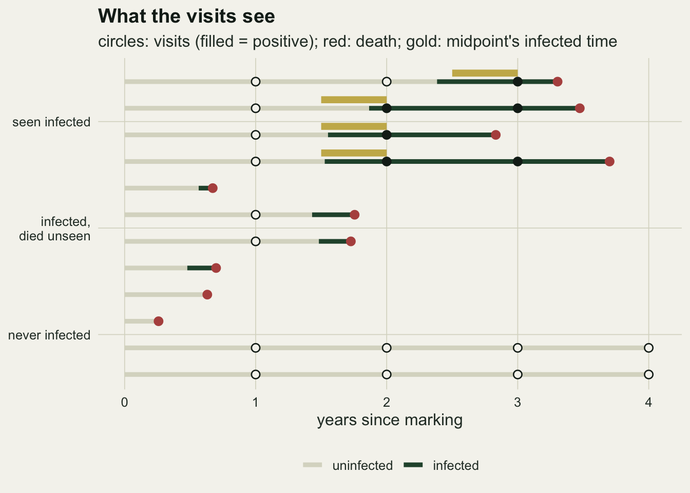
Two reflex codings and one hazard ratio
Both reflex codings put a change time into the (start, stop] layout of the source post and fit a Cox model. The detection-visit coding starts the infected interval at the first positive visit. The midpoint coding starts it half a visit interval earlier. A third fit, on the true change times that no field study has, is the reference.
cox_coded <- function(d, t_ch) {
  ch   <- t_ch < d$t_obs
  pre  <- data.frame(t0 = 0, t1 = ifelse(ch, t_ch, d$t_obs), ev = ifelse(ch, 0L, d$dead), x = 0L)
  post <- data.frame(t0 = t_ch[ch], t1 = d$t_obs[ch], ev = d$dead[ch], x = 1L)
  f <- coxph(Surv(t0, t1, ev) ~ x, data = rbind(pre, post))
  pt1 <- sum(post$t1 - post$t0); pt0 <- sum(pre$t1 - pre$t0)
  c(b = unname(coef(f)), s = sqrt(vcov(f)[1, 1]),
    rr = (sum(post$ev) / pt1) / (sum(pre$ev) / pt0), pt1 = pt1, pt0 = pt0)
}
ci_hr <- function(fit) exp(fit[["b"]] + c(0, -1.96, 1.96) * fit[["s"]])

fit_true <- cox_coded(cohort, cohort$t_change)
fit_det  <- cox_coded(cohort, cohort$t_detect)
fit_mid  <- cox_coded(cohort, cohort$t_mid)
hr_true_fit <- ci_hr(fit_true); hr_det <- ci_hr(fit_det); hr_mid <- ci_hr(fit_mid)
On the true change times the hazard ratio is 2.56 (95 per cent interval 1.97 to 3.33), against a truth of 3. The detection-visit coding gives 2.66 (1.95 to 3.63), and the midpoint coding 1.25 (0.94 to 1.65). The coding that looks more careful, because it puts the change in the middle of the interval where it is on average, is the one furthest from the truth.
The likelihood that uses only what was seen
The illness-death model has three states: uninfected (0), infected (1) and dead. With constant intensities, an animal leaves state 0 by infection at rate \(a\) or by death at rate \(h_0\), and dies in state 1 at rate \(h_1\); the hazard ratio is \(h_1 / h_0\). The probabilities of being in each live state after a stretch of length \(t\) have closed forms:
\[ P_{00}(t) = e^{-(a + h_0)t}, \qquad P_{11}(t) = e^{-h_1 t}, \qquad P_{01}(t) = \frac{a}{a + h_0 - h_1}\left(e^{-h_1 t} - e^{-(a + h_0)t}\right). \]
An animal’s likelihood is a product over what was seen. Each gap between two visits at which the animal was alive contributes \(P_{00}\), \(P_{01}\) or \(P_{11}\) for the two states observed. An animal still alive at four years ends on a visit and contributes nothing more. An animal that died \(r\) years after its last visit contributes \(P_{11}(r)\,h_1\) if that visit found it infected, and \(P_{00}(r)\,h_0 + P_{01}(r)\,h_1\) if it did not: it either died uninfected, or became infected unseen and died infected. That second term is the one both reflex codings get wrong. With a fixed visit grid every gap has the same length, so the gaps reduce to three counts, and the whole likelihood is vectorised.
idm_negll <- function(p, cnt, r_dead, s_dead, dv) {
  if (any(!is.finite(p)) || any(abs(p) > 30)) return(1e10)
  a <- exp(p[1]); h0 <- exp(p[2]); h1 <- exp(p[3]); dl <- a + h0 - h1
  P00 <- function(t) exp(-(a + h0) * t)
  P11 <- function(t) exp(-h1 * t)
  P01 <- function(t) a * exp(-h1 * t) * (if (abs(dl) < 1e-9) t else -expm1(-dl * t) / dl)
  ll <- cnt[1] * log(P00(dv)) + cnt[2] * log(P01(dv)) + cnt[3] * log(P11(dv)) +
    sum(log(ifelse(s_dead == 1, P11(r_dead) * h1, P00(r_dead) * h0 + P01(r_dead) * h1)))
  if (is.finite(ll)) -ll else 1e10
}

idm_starts <- list(log(c(0.4, 0.3, 0.3)), log(c(0.1, 1, 1)), log(c(1, 0.1, 3)))

fit_idm <- function(d, dv) {
  j <- ceiling(d$t_change / dv)   # used only through the visits: j <= n_vis exactly when seen
  cnt <- c(sum(ifelse(d$seen, j - 1, d$n_vis)),        # gaps 0 -> 0
           sum(d$seen),                                # gaps 0 -> 1
           sum(ifelse(d$seen, d$n_vis - j, 0)))        # gaps 1 -> 1
  dd <- d$dead == 1
  r_dead <- d$t_obs[dd] - d$n_vis[dd] * dv
  s_dead <- as.integer(d$seen[dd])
  fits <- lapply(idm_starts, function(st) optim(st, idm_negll, cnt = cnt, r_dead = r_dead,
                                                s_dead = s_dead, dv = dv, method = "BFGS"))
  vals <- sapply(fits, `[[`, "value")
  best <- fits[[which.min(vals)]]
  v <- solve(optimHess(best$par, idm_negll, cnt = cnt, r_dead = r_dead, s_dead = s_dead, dv = dv))
  c(b = best$par[3] - best$par[2], s = sqrt(v[3, 3] + v[2, 2] - 2 * v[2, 3]),
    spread = max(vals) - min(vals), conv = best$convergence,
    a = exp(best$par[1]), h0 = exp(best$par[2]))
}

fit_ill <- fit_idm(cohort, dv_demo)
hr_ill <- ci_hr(fit_ill)
The counts use the true change time only through the question of which visit first found the animal infected, which is what a field data sheet records. Fitted from three starting points, the three maxima agree to \(1.7 \times 10^{-6}\) in log-likelihood. The fitted hazard ratio is 4.12 (2.69 to 6.32), with an infection rate of 0.42 a year against 0.4 and a baseline death rate of 0.22 against 0.3. The interval comes from the inverse of the numerical Hessian, on the log scale. In this cohort the illness-death estimate lands above the truth by more than the true-time fit lands below it, and its interval is the widest of the four; it still contains 3. Not knowing the change times costs precision, and whether the estimator is also biased is a question one cohort cannot answer.
One cohort is one draw. The replicates below put numbers on all four fits.
Two hundred data sets per cell
The grid crosses three true hazard ratios (protective, none, harmful) with three visit intervals (six months, one year, two years), with the design otherwise as above. Each cell gets 200 fresh cohorts, a number fixed before any result was looked at. Coverage is the share of cohorts whose 95 per cent interval contains the true hazard ratio.
n_rep <- 200
hr_grid <- c(0.5, 1, 3); dv_grid <- c(0.5, 1, 2)

one_rep <- function(hr, dv) {
  d <- sim_panel(n_animal, hr, dv)
  ft <- cox_coded(d, d$t_change); fd <- cox_coded(d, d$t_detect); fm <- cox_coded(d, d$t_mid)
  fi <- fit_idm(d, dv)
  moved <- sum(d$t_detect[d$seen] - d$t_mid[d$seen])   # person-time the midpoint moves
  c(b_true = ft[["b"]], s_true = ft[["s"]], b_det = fd[["b"]], s_det = fd[["s"]],
    b_mid = fm[["b"]], s_mid = fm[["s"]], b_idm = fi[["b"]], s_idm = fi[["s"]],
    spread = fi[["spread"]], conv = fi[["conv"]],
    rr_det = fd[["rr"]], rr_mid = fm[["rr"]], pt1 = fd[["pt1"]], pt0 = fd[["pt0"]], moved = moved,
    n_seen = sum(d$seen), unseen = mean(d$t_change < d$t_obs & !d$seen))
}

cells <- expand.grid(dv = dv_grid, hr = hr_grid)
set.seed(60330)
reps <- lapply(seq_len(nrow(cells)), function(i)
  as.data.frame(t(replicate(n_rep, one_rep(cells$hr[i], cells$dv[i])))))

methods <- c(true = "true change time", det = "detection visit", mid = "midpoint", idm = "illness-death")
summ <- do.call(rbind, lapply(seq_len(nrow(cells)), function(i) {
  r <- reps[[i]]; hr <- cells$hr[i]
  do.call(rbind, lapply(names(methods), function(m) {
    b <- r[[paste0("b_", m)]]; s <- r[[paste0("s_", m)]]
    data.frame(hr = hr, dv = cells$dv[i], method = methods[[m]],
               med = exp(median(b)), q10 = exp(quantile(b, 0.1)), q90 = exp(quantile(b, 0.9)),
               cover = mean(abs(b - log(hr)) < 1.96 * s), reject = mean(abs(b / s) > 1.96))
  }))
}))
rownames(summ) <- NULL
cell_of <- function(hr, dv) which(cells$hr == hr & cells$dv == dv)
sv <- function(hr, dv, m, col = "med") summ[[col]][summ$hr == hr & summ$dv == dv & summ$method == methods[[m]]]
mcse <- function(p, n = n_rep) sqrt(p * (1 - p) / n)

idm_cover <- summ$cover[summ$method == methods[["idm"]]]
idm_ratio <- summ$med[summ$method == methods[["idm"]]] / summ$hr[summ$method == methods[["idm"]]]
spread_max <- max(sapply(reps, function(r) max(r$spread)))
n_nonconv  <- sum(sapply(reps, function(r) sum(r$conv != 0)))
unseen_of  <- function(hr, dv) median(reps[[cell_of(hr, dv)]]$unseen)
At the null, with yearly visits, the true-time fit has a median hazard ratio of 0.99, the detection-visit coding 1.01, the illness-death model 1.02, and the midpoint coding 0.57. The midpoint coding rejects the true null in 0.93 of the cohorts, against 0.04 for the detection visit and 0.05 for the illness-death model (Monte Carlo standard error about 0.015 near the nominal 0.05). With a true hazard ratio of 3 the detection visit gives 2.37, the midpoint 1.18 and the illness-death model 3.03, with coverage of 0.72, 0.00 and 0.96. A protective truth of 0.5 is not reversed by the midpoint coding but exaggerated, to 0.33.
Across all nine cells the illness-death model’s median sits between 0.98 and 1.04 times the truth, and its coverage runs from 0.93 to 0.98 (standard error about 0.015 at 0.95). The three starting points never disagreed by more than \(4.0 \times 10^{-3}\) in log-likelihood, and no fit reported non-convergence.
summ$method <- factor(summ$method, levels = unname(methods))
hr_labs <- sprintf("true HR %s", as.character(hr_grid))
summ$panel  <- factor(sprintf("true HR %s", as.character(summ$hr)), levels = hr_labs)
meth_cols <- setNames(c(te_body, te_gold, te_rust, te_forest), unname(methods))
meth_shapes <- setNames(c(1, 16, 16, 16), unname(methods))
truth_df <- data.frame(panel = factor(hr_labs, levels = hr_labs), hr = hr_grid)
dodge <- position_dodge(width = 0.6)
p_est <- ggplot(summ, aes(factor(dv), med, colour = method, shape = method)) +
  geom_hline(data = truth_df, aes(yintercept = hr), colour = te_ink, linetype = "dashed", linewidth = 0.5) +
  geom_errorbar(aes(ymin = q10, ymax = q90), width = 0, linewidth = 0.8, position = dodge) +
  geom_point(size = 2.4, stroke = 1, position = dodge) +
  facet_wrap(~ panel, scales = "free_y") +
  scale_y_log10() +
  scale_colour_manual(values = meth_cols, name = NULL) +
  scale_shape_manual(values = meth_shapes, name = NULL) +
  labs(x = NULL, y = "hazard ratio (log)",
       title = "The illness-death fit sits on the truth in every cell",
       subtitle = "dashed: the true hazard ratio") +
  theme_datasheet() + theme(legend.position = "none", strip.text = element_text(colour = te_ink, face = "bold"))
p_cov <- ggplot(summ, aes(factor(dv), cover, colour = method, shape = method)) +
  geom_hline(yintercept = 0.95, colour = te_ink, linetype = "dashed", linewidth = 0.5) +
  geom_point(size = 2.4, stroke = 1, position = dodge) +
  facet_wrap(~ panel) +
  scale_y_continuous(limits = c(0, 1)) +
  scale_colour_manual(values = meth_cols, name = NULL) +
  scale_shape_manual(values = meth_shapes, name = NULL) +
  labs(x = "years between visits", y = "coverage") +
  theme_datasheet() + theme(legend.position = "bottom", strip.text = element_blank())
p_est / p_cov + plot_layout(heights = c(1.4, 1)) + plot_annotation(theme = theme_datasheet())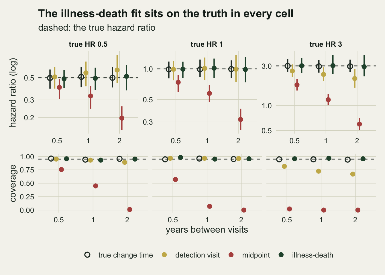
The two reflex codings fail in different ways, and the visit interval sets the size of both. The midpoint coding pulls every estimate down, and further the wider the interval: at the null its median is 0.74 with six-monthly visits and 0.32 with visits two years apart. With visits two years apart it turns a true hazard ratio of 3 into a median of 0.60, so an infection that triples mortality reads as protective. The detection-visit coding has medians between 0.99 and 1.01 at the null and shrinks a real effect towards one: at a true hazard ratio of 3 its median is 2.60, 2.37 and 2.11 from the shortest interval to the longest, and at a true 0.5 it is 0.51, 0.56 and 0.60.
The midpoint’s bias is person-time arithmetic
The direction of the midpoint’s bias follows from bookkeeping, and it helps to write it down before reading any more simulation. Take the detection-visit coding as the starting point, with \(D_1\) deaths in \(T_1\) years of infected follow-up and \(D_0\) deaths in \(T_0\) uninfected years. The midpoint coding moves every seen infection earlier by half an interval, so it moves \(I = n_\text{seen}\,\Delta/2\) years from the uninfected column to the infected one, where \(\Delta\) is the visit interval. It moves no death, because an animal seen infected at a visit was alive at that visit. The crude rate ratio becomes
\[ \frac{D_1 / (T_1 + I)}{D_0 / (T_0 - I)} = \frac{D_1 / T_1}{D_0 / T_0} \times \frac{T_1}{T_1 + I} \times \frac{T_0 - I}{T_0}, \]
and both factors on the right are below one in every data set. So the midpoint coding lowers the crude rate ratio below the detection-visit one whatever the truth is. Under the null, where the detection-visit ratio is near one, it manufactures protection. This is the source post’s immortal time again (Suissa 2008 gives the epidemiological account), in slices of half a visit interval: the animal had to survive to the visit to be seen infected, and the midpoint coding files the second half of that interval as infected time in which it could not die. It is the same mechanism Nevo and colleagues call a negative dependency between the imputed covariate and the event time.
all_reps <- do.call(rbind, reps)
pred_mid <- with(all_reps, rr_det * pt1 / (pt1 + moved) * (pt0 - moved) / pt0)
id_err   <- max(abs(pred_mid - all_reps$rr_mid))
moved_ok <- max(abs(all_reps$moved - all_reps$n_seen * rep(cells$dv, each = n_rep) / 2))
n_cox_lower <- sum(all_reps$b_mid < all_reps$b_det)
null_y <- reps[[cell_of(1, 1)]]
rr_mid_null  <- median(null_y$rr_mid)
cox_mid_null <- exp(median(null_y$b_mid))
share_cox_below_rr <- mean(exp(all_reps$b_mid) < all_reps$rr_mid)
Over all 1800 cohorts, the identity and the directly computed midpoint rate ratio agree to within floating-point rounding, and the moved time equals half an interval per seen infection exactly. It is an identity, not an approximation, and the simulation checks only that the code does what the algebra says.
The identity fixes the direction for a crude rate ratio. It does not fix the size of the Cox estimate. At the null with yearly visits the midpoint’s crude rate ratio has a median of 0.66, while the Cox estimate on the same coding has a median of 0.57; the Cox midpoint estimate falls below the crude one in 0.92 of all cohorts. The Cox midpoint estimate is below the Cox detection-visit estimate in every one of the 1800. The source post’s sentence can therefore be sharpened: the midpoint coding biases the change time in a known direction, and the hazard ratio too, towards protection.
null_df <- do.call(rbind, lapply(dv_grid, function(v) {
  r <- reps[[cell_of(1, v)]]
  data.frame(dv = sprintf("%s yr between visits", as.character(v)),
             pred = with(r, rr_det * pt1 / (pt1 + moved) * (pt0 - moved) / pt0),
             cox = exp(r$b_mid), det = exp(r$b_det))
}))
null_df$dv <- factor(null_df$dv, levels = sprintf("%s yr between visits", as.character(dv_grid)))
ggplot(null_df, aes(pred, cox, colour = dv)) +
  geom_abline(slope = 1, intercept = 0, colour = te_ink, linetype = "dashed", linewidth = 0.5) +
  geom_hline(yintercept = 1, colour = te_body, linewidth = 0.3) +
  geom_vline(xintercept = 1, colour = te_body, linewidth = 0.3) +
  geom_point(size = 1.3, alpha = 0.6) +
  scale_x_log10() + scale_y_log10() +
  scale_colour_manual(values = c(te_gold, te_forest, te_rust), name = NULL) +
  labs(x = "crude rate ratio predicted by the identity (log scale)",
       y = "Cox hazard ratio, midpoint coding (log scale)",
       title = "True hazard ratio 1, read through the midpoint",
       subtitle = "dashed: equality") +
  guides(colour = guide_legend(override.aes = list(size = 2.5, alpha = 1))) +
  theme_datasheet() + theme(legend.position = "bottom")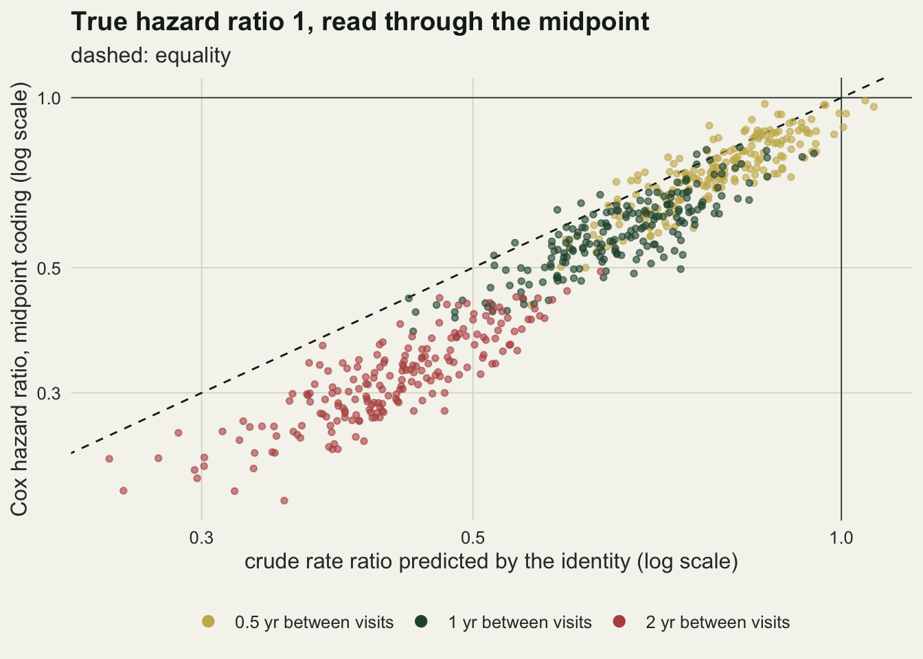
The detection visit loses the animals that die unseen
The detection-visit coding makes the covariate a function of the past: at any moment it records what the last visit found. Under the null the state does nothing to the hazard, so any such coding leaves the estimate unbiased, and it does here. With a real effect, the stretch between infection and detection is filed as uninfected time, and the deaths in it, including those of animals that die before any visit finds them infected, are filed as uninfected deaths. That stretch carries the infected death rate, so the uninfected column is a mixture of the two rates. With a harmful effect the mixture raises the uninfected rate and pulls the ratio down; with a protective one it lowers the uninfected rate and pulls the ratio up. Either way the estimate moves towards one, as the medians above show.
The share of animals infected but never seen infected is the size of that misfiling. It is 0.080 at the null with yearly visits and 0.197 at a true hazard ratio of 3, because an infection that raises mortality kills more animals before the next visit can find it. With visits two years apart and a true 3 it rises to 0.330, and with six-monthly visits it falls to 0.110. The illness-death likelihood gives each of those deaths the term \(P_{00}(r)\,h_0 + P_{01}(r)\,h_1\), which weighs both possibilities instead of choosing one.
The repair inherits its clock
Every rate in the simulation so far is constant, and the illness-death model above assumes the same. The Cox codings do not need that, because a Cox model compares animals at the same time since marking. The last cells let the baseline death rate rise with time since marking, as it does when marked adults age, with a cumulative hazard of \(0.3\,t^{1.6}\) instead of \(0.3\,t\), and the same proportional effect of infection. Two illness-death fits are compared: the constant-rate one above, and one whose death intensities have a Weibull shape, \(h_0(t) = \lambda k t^{k-1}\) and \(h_1(t) = \text{HR}\,h_0(t)\), with the infection rate still constant. The Weibull version has no closed form for \(P_{01}\), which becomes an integral over the unseen infection time,
\[ P_{01}(s, e) = \int_s^e P_{00}(s, u)\, a\, P_{11}(u, e)\, du, \]
computed below by 16-point Gauss-Legendre quadrature. The Weibull family matches the simulated shape by construction; the limits say what that buys.
gl_nodes <- function(m) {                      # Gauss-Legendre nodes and weights on [0, 1]
  b <- seq_len(m - 1) / sqrt(4 * seq_len(m - 1)^2 - 1)
  J <- matrix(0, m, m); J[cbind(1:(m - 1), 2:m)] <- b; J[cbind(2:m, 1:(m - 1))] <- b
  e <- eigen(J, symmetric = TRUE)
  list(x = (e$values + 1) / 2, w = e$vectors[1, ]^2)
}
gl16 <- gl_nodes(16)

wb_probs <- function(s, e, a, lam, k, hr) {
  cumh <- function(x, y) lam * (y^k - x^k)
  U <- outer(e - s, gl16$x) + s                # quadrature nodes, one row per stretch
  integrand <- exp(-a * (U - s) - cumh(s, U)) * a * exp(-hr * cumh(U, e))
  list(P00 = exp(-a * (e - s) - cumh(s, e)), P11 = exp(-hr * cumh(s, e)),
       P01 = as.numeric(integrand %*% gl16$w) * (e - s))
}
wb_negll <- function(p, dat) {
  if (any(!is.finite(p)) || any(abs(p) > 30)) return(1e10)
  a <- exp(p[1]); lam <- exp(p[2]); k <- exp(p[3]); hr <- exp(p[4])
  g <- wb_probs(dat$g_s, dat$g_e, a, lam, k, hr)
  f <- wb_probs(dat$d_s, dat$d_e, a, lam, k, hr)
  h0 <- lam * k * dat$d_e^(k - 1)
  lik_d <- ifelse(dat$d_st == 1, f$P11 * hr * h0, (f$P00 + f$P01 * hr) * h0)
  ll <- sum(dat$n00 * log(g$P00)) + sum(dat$n01 * log(g$P01)) + sum(dat$n11 * log(g$P11)) +
    sum(log(lik_d))
  if (is.finite(ll)) -ll else 1e10
}
fit_wb <- function(d, dv) {
  kk <- seq_len(round(tau_follow / dv)); j <- ceiling(d$t_change / dv); dd <- d$dead == 1
  dat <- list(g_s = (kk - 1) * dv, g_e = kk * dv,     # visit gaps are no longer interchangeable
              n00 = sapply(kk, function(k) sum(k <= ifelse(d$seen, j - 1, d$n_vis))),
              n01 = sapply(kk, function(k) sum(d$seen & j == k)),
              n11 = sapply(kk, function(k) sum(d$seen & k > j & k <= d$n_vis)),
              d_s = d$n_vis[dd] * dv, d_e = d$t_obs[dd], d_st = as.integer(d$seen[dd]))
  crude <- sum(d$dead) / sum(d$t_obs)
  starts <- list(c(log(0.4), log(crude), 0, 0), c(0, log(crude / 3), log(2), log(3)),
                 c(log(0.1), log(crude * 2), log(0.6), log(1 / 3)))
  fits <- lapply(starts, function(st) optim(st, wb_negll, dat = dat, method = "BFGS",
                                            control = list(maxit = 500)))
  vals <- sapply(fits, `[[`, "value"); best <- fits[[which.min(vals)]]
  v <- solve(optimHess(best$par, wb_negll, dat = dat))
  c(b = best$par[4], s = sqrt(v[4, 4]), k = exp(best$par[3]), spread = max(vals) - min(vals),
    a = exp(best$par[1]), lam = exp(best$par[2]))
}

n_rep_age <- 100
age_cells <- data.frame(shape = c(1.6, 1.6, 1), hr = c(1, 3, 3))
set.seed(60331)
age_reps <- lapply(seq_len(nrow(age_cells)), function(i) {
  as.data.frame(t(replicate(n_rep_age, {
    d <- sim_panel(n_animal, age_cells$hr[i], 1, age_cells$shape[i])
    fd <- cox_coded(d, d$t_detect); fm <- cox_coded(d, d$t_mid)
    fi <- fit_idm(d, 1); fw <- fit_wb(d, 1)
    c(b_det = fd[["b"]], s_det = fd[["s"]], b_mid = fm[["b"]], s_mid = fm[["s"]],
      b_idm = fi[["b"]], s_idm = fi[["s"]], b_wb = fw[["b"]], s_wb = fw[["s"]],
      k_wb = fw[["k"]], spread_wb = fw[["spread"]], a_wb = fw[["a"]], lam_wb = fw[["lam"]])
  })))
})
age_methods <- c(det = "detection visit", mid = "midpoint", idm = "illness-death, constant",
                 wb = "illness-death, Weibull")
age_summ <- do.call(rbind, lapply(seq_len(nrow(age_cells)), function(i) {
  r <- age_reps[[i]]; hr <- age_cells$hr[i]
  do.call(rbind, lapply(names(age_methods), function(m) {
    b <- r[[paste0("b_", m)]]; s <- r[[paste0("s_", m)]]
    data.frame(shape = age_cells$shape[i], hr = hr, method = age_methods[[m]],
               med = exp(median(b)), q10 = exp(quantile(b, 0.1)), q90 = exp(quantile(b, 0.9)),
               cover = mean(abs(b - log(hr)) < 1.96 * s))
  }))
}))
rownames(age_summ) <- NULL
av <- function(shape, hr, m, col = "med") age_summ[[col]][age_summ$shape == shape & age_summ$hr == hr &
                                                          age_summ$method == age_methods[[m]]]
k_med <- sapply(age_reps, function(r) median(r$k_wb))
wb_spread_max <- max(sapply(age_reps, function(r) max(r$spread_wb)))
haz_1 <- haz_base * 1.6 * 1^0.6; haz_4 <- haz_base * 1.6 * 4^0.6
width_ratio <- median(age_reps[[3]]$s_wb / age_reps[[3]]$s_idm)

# quadrature against integrate() at every fitted Weibull parameter set: the four visit gaps
# and the stretches of a quarter, half and three quarters of a year after each visit
quad_stretch <- expand.grid(s = 0:3, len = c(0.25, 0.5, 0.75, 1))
quad_relerr <- function(a, lam, k, hr) {
  q <- wb_probs(quad_stretch$s, quad_stretch$s + quad_stretch$len, a, lam, k, hr)$P01
  ex <- mapply(function(s, e) integrate(function(u) exp(-a * (u - s) - lam * (u^k - s^k)) * a *
                 exp(-hr * lam * (e^k - u^k)), s, e, rel.tol = 1e-10)$value,
               quad_stretch$s, quad_stretch$s + quad_stretch$len)
  max(abs(q - ex) / ex)
}
quad_err <- max(unlist(lapply(age_reps, function(r)
  mapply(quad_relerr, r$a_wb, r$lam_wb, r$k_wb, exp(r$b_wb)))))
n_quad_sets <- sum(sapply(age_reps, nrow))
The rising baseline death rate is 0.48 a year at one year after marking and 1.10 at four years. Each of the three cells below has 100 cohorts with yearly visits.
With that rising baseline and no effect of infection, the constant-rate illness-death model returns a median hazard ratio of 2.33, and with a true hazard ratio of 3 it returns 7.75; its coverage is 0.00 and 0.02. Infected animals are, on average, further into their follow-up than uninfected ones, and further into follow-up is where the deaths now are. A model with one death rate per state can only explain those deaths by the state. The two Cox codings do not see the problem: at the null the detection visit gives 1.02 and the midpoint 0.61, the same pattern as with constant rates.
The Weibull illness-death model gives 1.02 at the null and 3.12 at a true 3, with coverage 0.94 and 0.95, and a median fitted shape of 1.60 and 1.60 against the true 1.6. On cohorts with constant rates it gives 2.93 at a true 3 (coverage 0.97, fitted shape 1.01), where its standard error is a median 1.19 times that of the constant-rate fit on the same cohorts. Its three starts never disagreed by more than \(6.3 \times 10^{-5}\) in log-likelihood. At the fitted parameters of all 300 Weibull fits, the 16-point rule agrees with R’s integrate() over the four visit gaps and over stretches of a quarter, a half and three quarters of a year after each visit (a death term integrates over such a stretch, from the last visit to the death), to a relative error of at most \(1.9 \times 10^{-6}\).
age_summ$method <- factor(age_summ$method, levels = unname(age_methods))
age_levels <- c("rising baseline, true HR 1", "rising baseline, true HR 3", "constant baseline, true HR 3")
age_summ$panel <- factor(sprintf("%s baseline, true HR %s", ifelse(age_summ$shape == 1, "constant", "rising"),
                                 as.character(age_summ$hr)), levels = age_levels)
age_cols <- setNames(c(te_gold, te_rust, te_ink, te_forest), unname(age_methods))
age_shapes <- setNames(c(16, 16, 1, 16), unname(age_methods))
age_truth <- data.frame(panel = factor(age_levels, levels = age_levels), hr = c(1, 3, 3))
ggplot(age_summ, aes(method, med, colour = method, shape = method)) +
  geom_hline(data = age_truth, aes(yintercept = hr), colour = te_ink, linetype = "dashed", linewidth = 0.5) +
  geom_errorbar(aes(ymin = q10, ymax = q90), width = 0, linewidth = 0.9) +
  geom_point(size = 2.6, stroke = 1.1) +
  facet_wrap(~ panel) +
  scale_y_log10() +
  scale_colour_manual(values = age_cols, name = NULL) +
  scale_shape_manual(values = age_shapes, name = NULL) +
  labs(x = NULL, y = "estimated hazard ratio (log scale)",
       title = "A constant-rate repair breaks when mortality rises",
       subtitle = "dashed: the true hazard ratio") +
  guides(colour = guide_legend(nrow = 2)) +
  theme_datasheet() +
  theme(legend.position = "bottom", axis.text.x = element_blank(),
        strip.text = element_text(colour = te_ink, face = "bold"))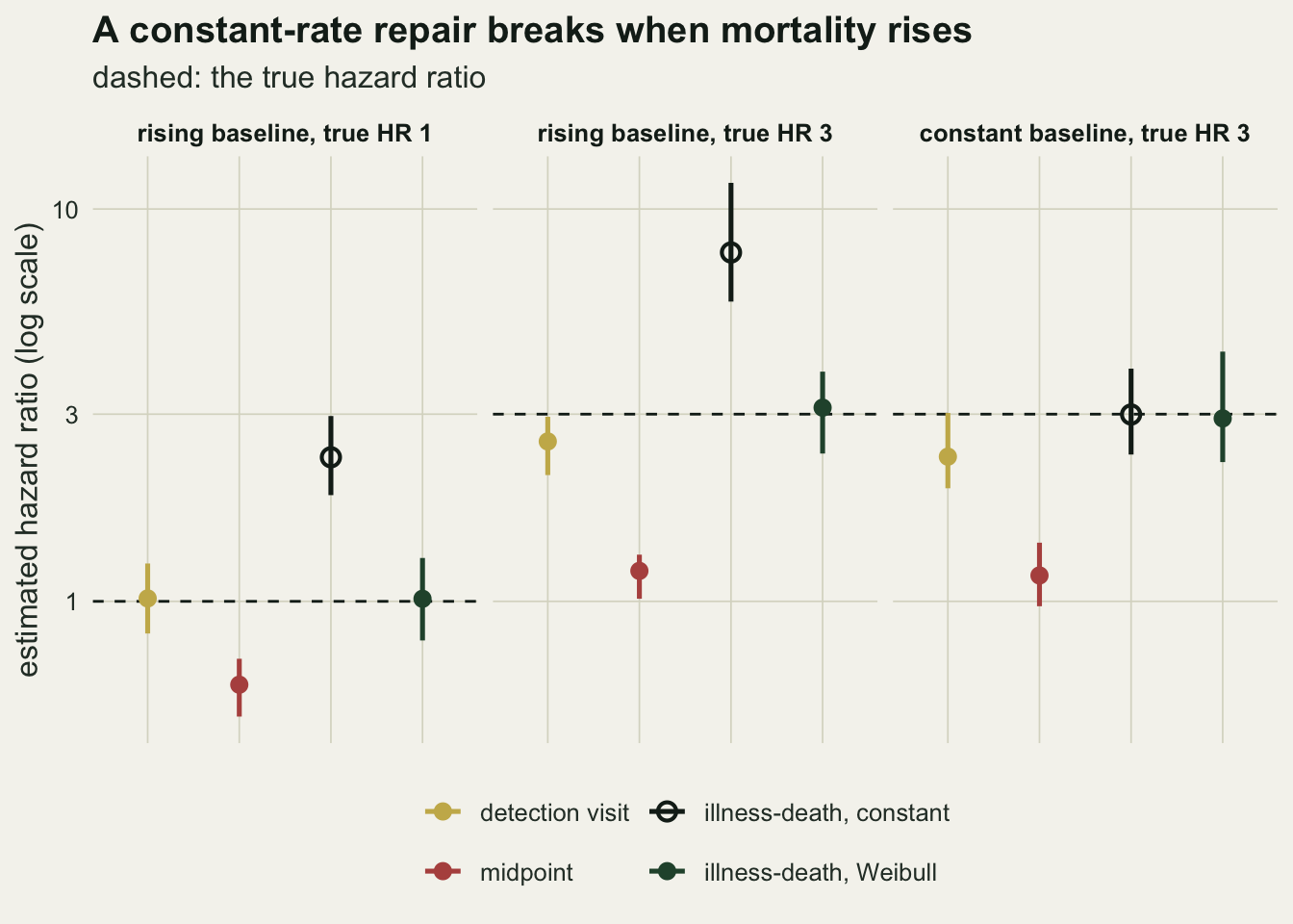
A shape of 1.6 is a steep rise. The chunk below asks how mild a rise the constant-rate fit survives, and fits only that model, which keeps it cheap: 100 fresh cohorts per cell, with shapes of 1.1, 1.2 and 1.3.
mild_cells <- expand.grid(hr = c(1, 3), shape = c(1.1, 1.2, 1.3))
set.seed(60332)
mild_reps <- lapply(seq_len(nrow(mild_cells)), function(i) as.data.frame(t(replicate(n_rep_age, {
  d <- sim_panel(n_animal, mild_cells$hr[i], 1, mild_cells$shape[i])
  fi <- fit_idm(d, 1)
  c(b = fi[["b"]], s = fi[["s"]])
}))))
mild_cells$med   <- sapply(mild_reps, function(r) exp(median(r$b)))
mild_cells$cover <- sapply(seq_along(mild_reps), function(i)
  mean(abs(mild_reps[[i]]$b - log(mild_cells$hr[i])) < 1.96 * mild_reps[[i]]$s))
mv <- function(shape, hr, col = "med") mild_cells[[col]][mild_cells$shape == shape & mild_cells$hr == hr]
rise_of <- function(shape) 4^(shape - 1)     # death rate at four years over the rate at one year
With the death rate at four years 1.15, 1.32 and 1.52 times the rate at one year, the constant-rate illness-death model returns median hazard ratios of 1.15, 1.33 and 1.54 at the null, with coverage 0.86, 0.61 and 0.29, and 3.64, 4.55 and 4.85 at a true 3, with coverage 0.83, 0.57 and 0.43. The bias grows with the rise, and the mildest one, a death rate 15 per cent higher at four years than at one, already puts both coverages below 0.95 by more than three times the Monte Carlo standard error of a coverage at 0.95 (about 0.022).
So the likelihood repairs the coding and imports a model of time in exchange. The Cox codings are wrong about the state and right about time; the constant-rate likelihood is right about the state and can be badly wrong about time. Joly and colleagues estimated the intensities by penalised likelihood, smooth and without a parametric shape, for this reason, and a Weibull shape is a small step in that direction.
What to report
Say how the state was observed: at which visits, how far apart, whether a visit could miss the state, and whether the state at death was known from the carcass. Give the number of changes seen, the number seen only at the final visit, and the number of deaths among animals whose last visit found them in the original state; those deaths are the ones every coding has to guess about.
Do not code the change at the midpoint of the visit interval in a Cox model. The crude rate ratio it gives is below the detection-visit one in every data set, by the identity above, its Cox estimate was below the detection-visit one in every cohort here, and at the null with yearly visits it rejected the true null in 0.93 of the cohorts here. If a detection-visit coding is used, report it as a test of the null that is valid, and an estimate of a real effect that is shrunk towards one by an amount that grows with the visit interval.
For an estimate, fit an illness-death likelihood to the states at the visits and the exact death times, and give the baseline intensities a shape that can follow time since marking. Report the time scale, the shape, the starting points and whether the fits from different starts agreed. Report the fitted change rate alongside the hazard ratio, because it is estimated from the same visits and a reader can check it against the prevalence at each visit.
Honest limits
The simulated change is one way, permanent and independent of everything else, and each test is perfect. Imperfect tests add misclassification on top of interval censoring, and an animal that tests falsely negative after a positive test breaks the counting used here; a multi-event model of the kind in multi-event models for uncertain states adds that observation layer to a forward likelihood at discrete occasions, and which of the two biases dominates in a real serology study was not measured. The visit schedule is fixed and the same for every animal. When animals are caught more often in some states, or trapping effort stops when an animal looks ill, the visit times carry information and the likelihood above would be missing a term.
The infection state at death is unknown in every cell. A necropsy that records it changes the death term of the likelihood from \(P_{00}(r)\,h_0 + P_{01}(r)\,h_1\) to one of its two parts, so the likelihood knows which state each animal died in though not when it changed, and gives the detection-visit coding a way to recover those deaths as infected ones; that case was not simulated. Confounding is also untouched: the animals that become infected are a random subset here, and the source post’s remark that no coding removes confounding by what predicts both the change and the death applies unchanged.
The Weibull repair was checked only where the truth is Weibull, which is the kindest case. Every animal here is marked at the same point of its life, so time since marking is the only clock; animals marked at mixed ages put a rising hazard on age instead, which the Cox codings on time since marking and the Weibull fit here both ignore. That needs age as the time scale with delayed entry, as in the age-specific intensities of Joly and colleagues, and it was not simulated. A baseline that rises and then falls would need splines or a piecewise shape, and neither is tested here; nor are the Cox model with change times imputed by Monte Carlo EM of Goggins and colleagues, or the calibration models of Nevo and colleagues, either of which may do as well for less code. The intervals for the illness-death fits are Wald intervals on the log scale from a numerical Hessian, and their coverage is only as good as the replicates show.
Replication is 200 cohorts per cell in the main grid and 100 in the ageing cells, so a coverage near 0.95 carries a Monte Carlo standard error of about 0.015 in the first and 0.022 in the second, and a difference of a few points between two coverages is not resolved here. All cohorts have 300 animals and four years of follow-up.
References
Goggins WB, Finkelstein DM, Zaslavsky AM 1999 Biometrics 55(2):445-451 (10.1111/j.0006-341X.1999.00445.x)
Joly P, Commenges D, Helmer C, Letenneur L 2002 Biostatistics 3(3):433-443 (10.1093/biostatistics/3.3.433)
Leffondre K, Touraine C, Helmer C, Joly P 2013 International Journal of Epidemiology 42(4):1177-1186 (10.1093/ije/dyt126)
Nevo D, Hamada T, Ogino S, Wang M 2020 Biostatistics 21(2):e148-e163 (10.1093/biostatistics/kxy063)
Suissa S 2008 American Journal of Epidemiology 167(4):492-499 (10.1093/aje/kwm324)