Delayed entry and the Weibull hazard shape

Fitting a Weibull to animals first marked as adults, without their entry ages, inflates the shape and can turn juvenile mortality into senescence. Fixed in R.

A long-term study of a lizard population catches animals on a fixed set of plots and reads the age of each one from growth rings in a clipped toe bone, a method called skeletochronology. Every animal is then followed until it dies or the study ends. The data sheet has an age at death, or an age at the last sighting, for several hundred animals, and the question the study was set up to answer is whether the risk of dying rises with age. A Weibull model answers that in one parameter, its shape: above one the hazard rises with age, which is what senescence looks like in a survival curve; below one it falls, which is what heavy mortality of the young looks like. The age column goes into survreg, and a shape comes out, as the reciprocal of what survreg calls its scale.

The catch is in who is on the data sheet. An animal first caught at age three is on it because it was alive at age three. Its siblings that died at one and two were never caught, never aged and never entered anywhere. The sample is the lifetimes of animals that survived to be marked, which is left truncation, or delayed entry in the language of survival analysis. Its likelihood is textbook material: each animal contributes its density at the age of death divided by the probability of surviving to the age at which it entered, as set out by Klein and Moeschberger (2003) and Kalbfleisch and Prentice (2002). The direction of the damage when the division is left out is also standard. The early deaths are missing, the lifetimes that remain are longer than the population’s, and a fit that does not know why reads the shortage of early deaths as a property of the animals. Colchero and Clark (2012) built the same conditioning on survival to first capture, together with censoring, into a Bayesian capture-recapture model for wild animals of unknown birth year (Soay sheep), and their paper is the ecological source for the problem treated here in its simplest form. This post is a demonstration of that known result. What it measures are the parts a reader with a data sheet needs in numbers: which Weibull parameter carries the damage, whether the direction of the hazard itself can change, and how wide the spread of entry ages must be before any of it matters.

There is an honest reason the error is common, and it is not carelessness. The survival package, which is where most ecologists fit a Weibull, accepts an entry time for Cox models and for Kaplan-Meier curves but not for survreg; handed the three-column Surv(entry, age, dead) object, survreg stops with an error. The naive fit below is what an analyst gets from the standard tool after dropping the column the tool refused.

The site has met the arithmetic before. Lost collar signals and informative censoring already divides a Weibull density by the probability of surviving to retrieval, and finds a few per cent of optimism in the scale. Do the same arithmetic to the animals rather than the instruments and the damaged parameter is the shape, where a few per cent becomes an error of the same order as the parameter itself, and where the sign of the biological conclusion can flip. In that post the truncated fit is a way of building a battery curve for another likelihood, and the shape it estimates is computed and then left out of the table; here the truncation is the study design, since marking animals of mixed age is what most field studies do, and the shape is the answer. The closest cousin is interval-censored survival from visit data, which has already shown a falling Weibull hazard read as a rising one. There the cause was a coding of death dates found on tracking visits, every animal entered at release, and the repair was the interval likelihood. Here every death time is exact and correctly coded; the shortage of early deaths comes from which animals got into the study, and the repair is a column of entry ages.

Two other posts sit nearby and do not overlap. Time-varying covariates in a survival model is about immortal time inside animals that were all enrolled at time zero: its estimand is a hazard ratio, and its repair is the counting-process coding of each animal’s own history. The post on Kaplan-Meier survival curves assumes every animal is followed from the start, which is the assumption dropped here. The nearest post in spirit is transients and the single-capture rule in CJS, where animals are also missing from what the survival model sees. The difference is who removed them. In this post the missing animals were never in the study and nobody chose anything; in the transients post they were in the study and an analyst threw them out. That post’s repair is a change of model, and this one’s is a change of likelihood.

library(ggplot2)
library(patchwork)
library(survival)

te_paper  <- "#f5f4ee"
te_ink    <- "#16241d"
te_body   <- "#2c3a31"
te_forest <- "#275139"
te_rust   <- "#b5534e"
te_gold   <- "#c9b458"
te_line   <- "#dad9ca"

theme_datasheet <- function() {
  theme_minimal(base_size = 12) +
    theme(plot.background  = element_rect(fill = te_paper, colour = NA),
          panel.background = element_rect(fill = te_paper, colour = NA),
          panel.grid.major = element_line(colour = te_line, linewidth = 0.3),
          panel.grid.minor = element_blank(),
          text             = element_text(colour = te_body),
          plot.title       = element_text(colour = te_ink, face = "bold"),
          plot.subtitle    = element_text(colour = te_body),
          axis.text        = element_text(colour = te_body))
}

Only the animals still alive get marked

Lifetimes in years are drawn from a Weibull with scale 6. Each candidate animal is also given a marking age, drawn uniformly between zero and an upper limit, and it enters the data set only if it is still alive at that age. Candidates are drawn until the data set holds the required number of animals, so the sample size below always counts animals retained, never animals simulated. Every retained animal is followed to death or to age 12, whichever comes first. These constants, the grid of true shapes and entry windows, and the number of simulated data sets per cell were all fixed before any run.

wb_scale  <- 6
age_cens  <- 12
n_keep    <- 700
n_small   <- 200
shape_set <- c(0.5, 0.7, 1.0, 1.6, 2.2, 3.0)
entry_set <- c(0.5, 2, 5, 8)
n_draw    <- 200

sim_marked <- function(n_animals, shape, entry_max) {
  life <- entry <- numeric(0)
  while (length(life) < n_animals) {
    n_cand <- 3 * n_animals
    e_cand <- runif(n_cand, 0, entry_max)
    l_cand <- rweibull(n_cand, shape, wb_scale)
    alive  <- l_cand > e_cand
    life   <- c(life, l_cand[alive])
    entry  <- c(entry, e_cand[alive])
  }
  life <- life[seq_len(n_animals)]
  list(age = pmin(life, age_cens), dead = as.numeric(life <= age_cens),
       entry = entry[seq_len(n_animals)])
}

# share of candidates that die before their marking age, exact for the design
discard_share <- function(shape, entry_max) {
  1 - integrate(function(e) pweibull(e, shape, wb_scale, lower.tail = FALSE),
                0, entry_max)$value / entry_max
}

wb_median <- function(shape, scl) scl * log(2)^(1 / shape)
wb_hazard <- function(age, shape, scl) (shape / scl) * (age / scl)^(shape - 1)

Both fits use one likelihood with a switch. With shape k and scale s, a death at age a contributes the log density, a survivor at age 12 contributes the log survival probability, and the switch adds back the log survival probability at the entry age for every animal. That last term is the whole repair. The gradient is written out only so that thousands of fits run quickly; it plays no part in the argument.

nll_weib <- function(par, age, dead, entry, trunc) {
  k <- exp(par[1]); s <- exp(par[2])
  -sum(dead * (log(k) - k * log(s) + (k - 1) * log(age))) +  # deaths
    sum((age / s)^k) -                                         # minus log S(age), everyone
    trunc * sum((entry / s)^k)                                 # the repair: divide by S(entry)
}

grad_weib <- function(par, age, dead, entry, trunc) {
  k <- exp(par[1]); b <- par[2]
  lt <- log(age) - b; le <- log(entry) - b
  zt <- exp(k * lt);  ze <- exp(k * le)
  c(-sum(dead * (1 + k * lt)) + k * sum(zt * lt) - trunc * k * sum(ze * le),
    k * sum(dead) - k * sum(zt) + trunc * k * sum(ze))
}

fit_weib <- function(dat, trunc) {
  fit <- optim(c(0, log(median(dat$age))), nll_weib, grad_weib,
               age = dat$age, dead = dat$dead, entry = dat$entry, trunc = trunc,
               method = "BFGS", control = list(reltol = 1e-12))
  exp(fit$par)
}

One data set shows the two fits side by side. The true shape is 0.7, so the hazard falls with age and is highest in the first months of life, and animals are marked at ages spread evenly between zero and five years.

shape_anchor <- 0.7
entry_anchor <- 5
set.seed(2711)
worked   <- sim_marked(n_keep, shape_anchor, entry_anchor)
fit_nv   <- fit_weib(worked, trunc = 0)
fit_tr   <- fit_weib(worked, trunc = 1)
disc_one <- discard_share(shape_anchor, entry_anchor)
med_true_anchor <- wb_median(shape_anchor, wb_scale)

survreg_msg <- tryCatch(
  survreg(Surv(entry, age, dead) ~ 1, data = as.data.frame(worked), dist = "weibull"),
  error = function(e) conditionMessage(e))

Under this design a share of 0.387 of all candidate animals die before their marking age and never appear. The 700 that do give a naive shape of 1.345 and a truncated shape of 0.679, against a true 0.7. The naive median lifespan is 8.58 years and the truncated one 3.68, against a true 3.55. Asked to fit the same data with the entry column, survreg replies: “start-stop type Surv objects are not supported”.

The damage sits in the shape

One data set proves nothing about an estimator, so each combination of true shape, entry window and sample size is simulated 200 times, with both fits on every data set. Every per cent figure below is the median over those data sets of the estimate divided by the true value, minus one; the denominator is always the true parameter, not the corrected estimate.

cells <- expand.grid(shape = shape_set, entry_max = entry_set, n_animals = c(n_keep, n_small))
set.seed(5087)
draws <- lapply(seq_len(nrow(cells)), function(i) {
  out <- t(replicate(n_draw, {
    dat <- sim_marked(cells$n_animals[i], cells$shape[i], cells$entry_max[i])
    c(fit_weib(dat, 0), fit_weib(dat, 1))
  }))
  colnames(out) <- c("k_nv", "s_nv", "k_tr", "s_tr")
  out
})

pct_err <- function(est, truth) 100 * (median(est) / truth - 1)
mc_se_med <- function(est, truth) 100 * 1.2533 * sd(est / truth) / sqrt(length(est))

grid_tab <- do.call(rbind, lapply(seq_len(nrow(cells)), function(i) {
  a  <- draws[[i]]; sh <- cells$shape[i]
  mt <- wb_median(sh, wb_scale)
  med_nv <- wb_median(a[, "k_nv"], a[, "s_nv"])
  med_tr <- wb_median(a[, "k_tr"], a[, "s_tr"])
  data.frame(cells[i, ], discard = discard_share(sh, cells$entry_max[i]),
             k_nv = median(a[, "k_nv"]), k_tr = median(a[, "k_tr"]),
             k_nv_pct = pct_err(a[, "k_nv"], sh), k_tr_pct = pct_err(a[, "k_tr"], sh),
             k_tr_se = mc_se_med(a[, "k_tr"], sh),
             m_nv_pct = pct_err(med_nv, mt), m_tr_pct = pct_err(med_tr, mt),
             m_tr_se = mc_se_med(med_tr, mt), m_tr_sd = 100 * sd(med_tr / mt),
             flip = mean(a[, "k_nv"] > 1), flip_tr = mean(a[, "k_tr"] > 1))
}))

gcell <- function(sh, em, nn = n_keep) {
  grid_tab[grid_tab$shape == sh & grid_tab$entry_max == em & grid_tab$n_animals == nn, ]
}
anchor_rows <- grid_tab[grid_tab$entry_max == entry_anchor & grid_tab$n_animals == n_keep, ]

The table holds the entry window of the worked example, zero to five years, at 700 animals, for every true shape.

show_tab <- anchor_rows[, c("shape", "discard", "k_nv", "k_tr", "k_nv_pct", "m_nv_pct", "m_tr_pct")]
show_tab$discard <- 100 * show_tab$discard
names(show_tab) <- c("true shape", "candidates never marked, per cent", "naive shape",
                     "truncated shape", "naive shape error, per cent",
                     "naive median lifespan error, per cent",
                     "truncated median lifespan error, per cent")
knitr::kable(show_tab, digits = c(1, 1, 3, 3, 1, 1, 1), row.names = FALSE)

true shape	candidates never marked, per cent	naive shape	truncated shape	naive shape error, per cent	naive median lifespan error, per cent	truncated median lifespan error, per cent
0.5	44.3	1.170	0.493	134.1	250.0	-1.4
0.7	38.7	1.340	0.701	91.4	127.2	-0.6
1.0	32.2	1.596	0.997	59.6	64.7	0.2
1.6	23.1	2.131	1.598	33.2	26.4	-0.3
2.2	17.4	2.700	2.203	22.7	14.2	0.0
3.0	12.4	3.490	3.013	16.3	7.6	0.2

a_row <- function(sh) anchor_rows[anchor_rows$shape == sh, ]
k_nv_pct_all <- anchor_rows$k_nv_pct
k_tr_worst   <- max(abs(anchor_rows$k_tr_pct))

On a constant hazard, true shape 1.0, the naive fit returns a shape of 1.596, 59.6 per cent too high, and a median lifespan 64.7 per cent too long. A population in which the risk of dying does not change with age is reported as one that ages. At the worked example’s true shape of 0.7 the naive shape is 1.340, 91.4 per cent high, and the median lifespan is 127.2 per cent too long. At the steepest juvenile mortality in the grid, shape 0.5, the naive shape is 1.170.

The damage shrinks as the true shape rises: the naive shape error is 33.2, 22.7 and 16.3 per cent at true shapes of 1.6, 2.2 and 3.0, and the median lifespan error 26.4, 14.2 and 7.6 per cent. The reason is visible in the discard column. When the hazard rises steeply, few animals die before the age of marking, so there is little missing to misread; when it falls, the hazard is highest at the youngest ages, and the deaths there are exactly the deaths the design never sees. The truncated likelihood returns the shape to within 1.4 per cent at every true shape in the table.

age_seq <- seq(0.1, age_cens, length.out = 120)
haz_df <- do.call(rbind, lapply(shape_set, function(sh) {
  a <- draws[[which(cells$shape == sh & cells$entry_max == entry_anchor &
                     cells$n_animals == n_keep)]]
  h_nv <- apply(sapply(seq_len(nrow(a)), function(j) wb_hazard(age_seq, a[j, "k_nv"], a[j, "s_nv"])), 1, median)
  h_tr <- apply(sapply(seq_len(nrow(a)), function(j) wb_hazard(age_seq, a[j, "k_tr"], a[j, "s_tr"])), 1, median)
  rbind(data.frame(age = age_seq, haz = wb_hazard(age_seq, sh, wb_scale), fit = "true hazard"),
        data.frame(age = age_seq, haz = h_nv, fit = "naive fit"),
        data.frame(age = age_seq, haz = h_tr, fit = "truncated fit"))
}))
haz_df$panel <- factor(rep(sprintf("true shape %.1f", shape_set), each = 3 * length(age_seq)),
                       levels = sprintf("true shape %.1f", shape_set))

haz_df$fit <- factor(haz_df$fit, levels = c("truncated fit", "naive fit", "true hazard"))
haz_df <- haz_df[order(haz_df$fit), ]

ggplot(haz_df, aes(age, haz, colour = fit, linetype = fit, linewidth = fit,
                   group = interaction(fit, panel))) +
  geom_line() +
  facet_wrap(~ panel, nrow = 2, scales = "free_y") +
  scale_y_log10(labels = function(x) formatC(x, format = "fg", digits = 2)) +
  scale_colour_manual(values = c(te_forest, te_rust, te_ink), name = NULL) +
  scale_linetype_manual(values = c("solid", "solid", "22"), name = NULL) +
  scale_linewidth_manual(values = c(2.2, 1, 0.7), name = NULL) +
  labs(x = "age (years)", y = "hazard per year (log scale)",
       title = "Without the entry ages, a falling hazard rises",
       subtitle = "marking ages uniform between 0 and 5 years; 700 animals retained") +
  theme_datasheet() +
  theme(legend.position = "bottom",
        strip.text = element_text(colour = te_ink, face = "bold"))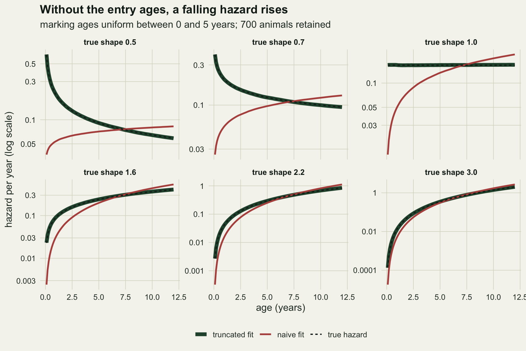

Figure 1: Pointwise median over 200 data sets of the fitted Weibull hazard, naive and truncated, against the true hazard, for six true shapes; animals marked between ages 0 and 5, 700 retained.

Below one, the sign of the answer changes

For a true shape above one the naive fit exaggerates a hazard that really does rise. Below one it does something of a different kind: it reports a rising hazard for a population whose hazard falls, which turns juvenile mortality into senescence. The question for a reader is how often that happens in a single study, not in the median over many.

flip_anchor <- gcell(shape_anchor, entry_anchor)$flip
flip_half   <- gcell(0.5, entry_anchor)$flip
flip_tr_max <- max(grid_tab$flip_tr[grid_tab$shape < 1])
flip_se     <- function(p) sqrt(p * (1 - p) / n_draw)

At true shape 0.7 with marking ages up to 5 years, the naive shape exceeds one in a share of 1.000 of the 200 data sets. At true shape 0.5 the share is 1.000. In no cell with a true shape below one does the truncated fit exceed one in more than 0.015 of data sets.

How much spread in entry ages before it matters

A study that marks every animal within its first months looks as if it has almost no truncation, and a study that marks animals at any age up to eight years has a great deal. The spread of entry ages, not the true shape alone, is what tells a reader whether their own study is affected, and it is the one thing about the design that the data sheet records.

yr_row  <- function(sh) gcell(sh, min(entry_set))
flip_by_entry <- sapply(entry_set, function(em) gcell(shape_anchor, em)$flip)
flip_half_by  <- sapply(entry_set, function(em) gcell(0.5, em)$flip)
k_nv_small_anchor <- gcell(shape_anchor, entry_anchor, n_small)$k_nv_pct
flip_small_anchor <- gcell(shape_anchor, entry_anchor, n_small)$flip
diff_n <- max(abs(grid_tab$k_nv_pct[grid_tab$n_animals == n_keep] -
                  grid_tab$k_nv_pct[grid_tab$n_animals == n_small]))

With every animal marked before half a year of age, the naive shape error is 0.0 per cent at true shape 3.0 and 2.7 per cent at 1.6, but already 12.3 per cent on a constant hazard, 27.6 per cent at 0.7 and 51.6 per cent at 0.5. When the hazard is steepest at birth, even a few months of unrecorded life before marking remove 17.3 per cent of all candidates, who die before they can be marked, at true shape 0.5.

The sign flip needs more spread. At true shape 0.7 the naive shape exceeds one in shares of 0.000, 1.000, 1.000 and 1.000 of data sets for entry windows of 0.5, 2, 5 and 8 years. At true shape 0.5, where the naive fit starts from further below one, the shares are 0.000, 0.135, 1.000 and 1.000.

Sample size does not enter the bias. With 200 animals instead of 700, the naive shape error at the worked design is 92.7 per cent and the flip share 1.000; across all 24 combinations of shape and entry window the two sample sizes differ by at most 2.0 percentage points in the naive shape error. A larger study measures the wrong shape more precisely.

sp_df <- grid_tab[grid_tab$n_animals == n_keep, ]
sp_long <- rbind(data.frame(sp_df[, c("shape", "entry_max")], k = sp_df$k_nv, fit = "naive fit, no entry ages"),
                 data.frame(sp_df[, c("shape", "entry_max")], k = sp_df$k_tr, fit = "truncated fit, with entry ages"))
sp_long$fit <- factor(sp_long$fit, levels = c("naive fit, no entry ages", "truncated fit, with entry ages"))
sp_long$true_lab <- factor(sprintf("true %.1f", sp_long$shape), levels = sprintf("true %.1f", shape_set))
shape_cols <- colorRampPalette(c(te_gold, te_rust, te_forest, te_ink))(length(shape_set))
lab_df <- sp_long[sp_long$entry_max == max(entry_set), ]
lab_df$vj <- ifelse(lab_df$fit == levels(sp_long$fit)[2], -0.6, 0.5)  # right panel: above the line

p_spread <- ggplot(sp_long, aes(entry_max, k, colour = true_lab)) +
  geom_hline(yintercept = 1, colour = te_body, linetype = "dashed", linewidth = 0.5) +
  geom_line(linewidth = 0.9) +
  geom_point(size = 2.2) +
  geom_text(data = lab_df, aes(label = true_lab, vjust = vj),
            hjust = 0, nudge_x = 0.35, size = 3.3, show.legend = FALSE) +
  facet_wrap(~ fit, nrow = 1) +
  scale_colour_manual(values = shape_cols, guide = "none") +
  scale_x_continuous(breaks = entry_set, limits = c(0.3, 11)) +
  scale_y_log10(breaks = c(0.5, 0.7, 1, 1.6, 2.2, 3)) +
  labs(x = "marking ages drawn uniformly from 0 to this age (years)",
       y = "median fitted shape (log scale)",
       title = "Without entry ages, a wider window means steeper ageing",
       subtitle = "one line per true shape; dashed: constant hazard") +
  theme_datasheet() +
  theme(strip.text = element_text(colour = te_ink, face = "bold"),
        panel.spacing.x = unit(1.2, "lines"))
p_spread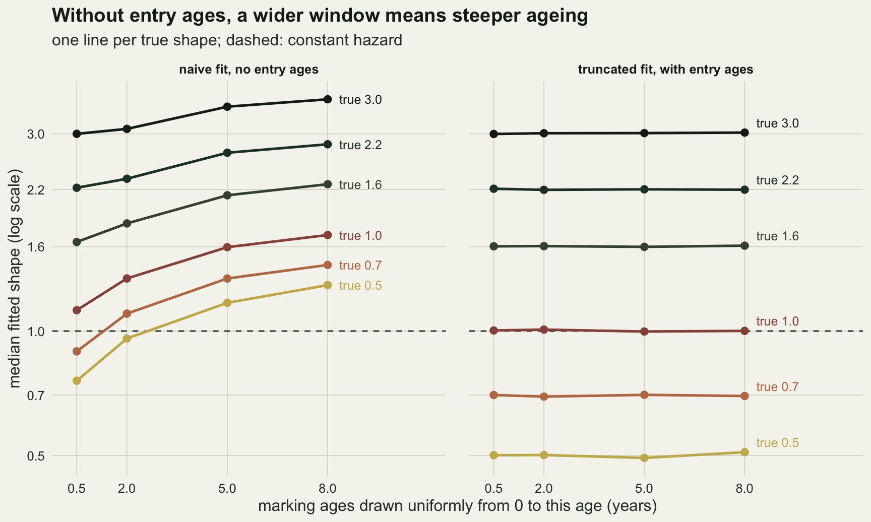

Figure 2: Median fitted Weibull shape over 200 data sets against the upper limit of the marking-age window, one line per true shape, for the naive fit (left) and the truncated fit (right); 700 animals retained.

A one-line check with the survival package

survreg refuses the entry column, but the Nelson-Aalen estimate of the cumulative hazard accepts it: survfit(Surv(entry, age, dead) ~ 1) returns it, and it is the same curve as the baseline hazard of the null Cox model coxph(Surv(entry, age, dead) ~ 1). For a Weibull the log cumulative hazard is a straight line in log age with the shape as its slope, which is the old Weibull plot. Fitting that line needs no parametric software, and it can be done with and without the entry ages. To keep the youngest ages, where only a handful of animals have entered, from dominating the line, only ages with at least 50 animals at risk are used; that threshold was fixed before the runs.

min_risk <- 50
weib_slope <- function(sf) {
  ok <- sf$cumhaz > 0 & sf$n.risk >= min_risk
  unname(coef(lm(log(sf$cumhaz[ok]) ~ log(sf$time[ok])))[2])
}
sf_nv_w <- survfit(Surv(worked$age, worked$dead) ~ 1)
sf_tr_w <- survfit(Surv(worked$entry, worked$age, worked$dead) ~ 1)
bh_w    <- basehaz(coxph(Surv(worked$entry, worked$age, worked$dead) ~ 1), centered = FALSE)
bh_gap  <- max(abs(bh_w$hazard - sf_tr_w$cumhaz[match(bh_w$time, sf_tr_w$time)]))

set.seed(3301)
cox_runs <- t(replicate(n_draw, {
  dat <- sim_marked(n_keep, shape_anchor, entry_anchor)
  c(ml_nv = fit_weib(dat, 0)[1], ml_tr = fit_weib(dat, 1)[1],
    na_nv = weib_slope(survfit(Surv(dat$age, dat$dead) ~ 1)),
    na_tr = weib_slope(survfit(Surv(dat$entry, dat$age, dat$dead) ~ 1)))
}))
colnames(cox_runs) <- c("ml_nv", "ml_tr", "na_nv", "na_tr")
cox_med  <- apply(cox_runs, 2, median)
cox_flip <- colMeans(cox_runs > 1)
cox_sd   <- apply(cox_runs, 2, sd)

In the worked data set the Cox baseline and the Nelson-Aalen curve agree to within floating-point rounding, and the slope of the Weibull plot is 1.481 without the entry ages and 0.797 with them. Over 200 fresh data sets at the same design, the median slope is 1.452 without the entry column and 0.728 with it, against 1.335 and 0.690 from the two likelihood fits to the same data. The slope without entry ages exceeds one in a share of 1.000 of data sets and the slope with them in 0.005. The graphical check shows the same reversal and the same repair, with a spread across data sets of 0.118 in the corrected slope against 0.063 for the corrected likelihood.

est_lab <- c(ml_nv = "likelihood, no entry ages", na_nv = "Nelson-Aalen slope, no entry ages",
             ml_tr = "likelihood, with entry ages", na_tr = "Nelson-Aalen slope, with entry ages")
draw_df <- do.call(rbind, lapply(names(est_lab), function(nm)
  data.frame(est = cox_runs[, nm], method = est_lab[[nm]],
             entry_used = ifelse(grepl("tr", nm), "with entry ages", "without entry ages"))))
draw_df$method <- factor(draw_df$method, levels = rev(unname(est_lab)))

ggplot(draw_df, aes(est, method, colour = entry_used)) +
  geom_vline(xintercept = 1, colour = te_body, linewidth = 0.5) +
  geom_vline(xintercept = shape_anchor, colour = te_body, linetype = "dashed", linewidth = 0.5) +
  geom_jitter(height = 0.18, width = 0, size = 1.1, alpha = 0.55) +
  scale_colour_manual(values = c("with entry ages" = te_forest, "without entry ages" = te_rust),
                      name = NULL) +
  labs(x = "estimated Weibull shape", y = NULL,
       title = "Juvenile mortality read as ageing, in every data set",
       subtitle = "dashed: true shape 0.7; solid: shape 1, constant hazard") +
  theme_datasheet() +
  theme(legend.position = "bottom")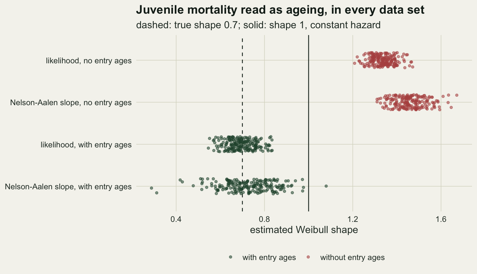

Figure 3: Shape estimates from 200 data sets with true shape 0.7 and marking ages up to 5 years: two Weibull likelihood fits and two Weibull-plot slopes from the Nelson-Aalen curve, each without and with the entry ages.

The Kaplan-Meier curve takes the entry column in the same way, and one data set shows what the naive curve does. Without entry ages it starts every animal at age zero, so the animals marked late count as survivors through ages at which nobody was watching them.

km_df <- rbind(
  data.frame(age = c(0, sf_nv_w$time), surv = c(1, sf_nv_w$surv), curve = "Kaplan-Meier, no entry ages"),
  data.frame(age = c(0, sf_tr_w$time), surv = c(1, sf_tr_w$surv), curve = "Kaplan-Meier, with entry ages"))
age_full <- seq(0, age_cens, length.out = 241)
true_df <- data.frame(age = age_full, surv = pweibull(age_full, shape_anchor, wb_scale, lower.tail = FALSE))
first_death_tr <- sf_tr_w$time[which(sf_tr_w$n.event > 0)[1]]
lost_before <- pweibull(first_death_tr, shape_anchor, wb_scale)
risk_first  <- sf_tr_w$n.risk[which(sf_tr_w$n.event > 0)[1]]

ggplot(km_df, aes(age, surv, colour = curve)) +
  geom_line(data = true_df, aes(age, surv), inherit.aes = FALSE,
            colour = te_ink, linetype = "dashed", linewidth = 0.8) +
  geom_step(linewidth = 0.8) +
  scale_colour_manual(values = c(te_rust, te_forest), name = NULL) +
  coord_cartesian(ylim = c(0, 1)) +
  labs(x = "age (years)", y = "proportion surviving",
       title = "The early deaths the design never saw",
       subtitle = "dashed: true survival, shape 0.7, scale 6") +
  theme_datasheet() +
  theme(legend.position = "bottom")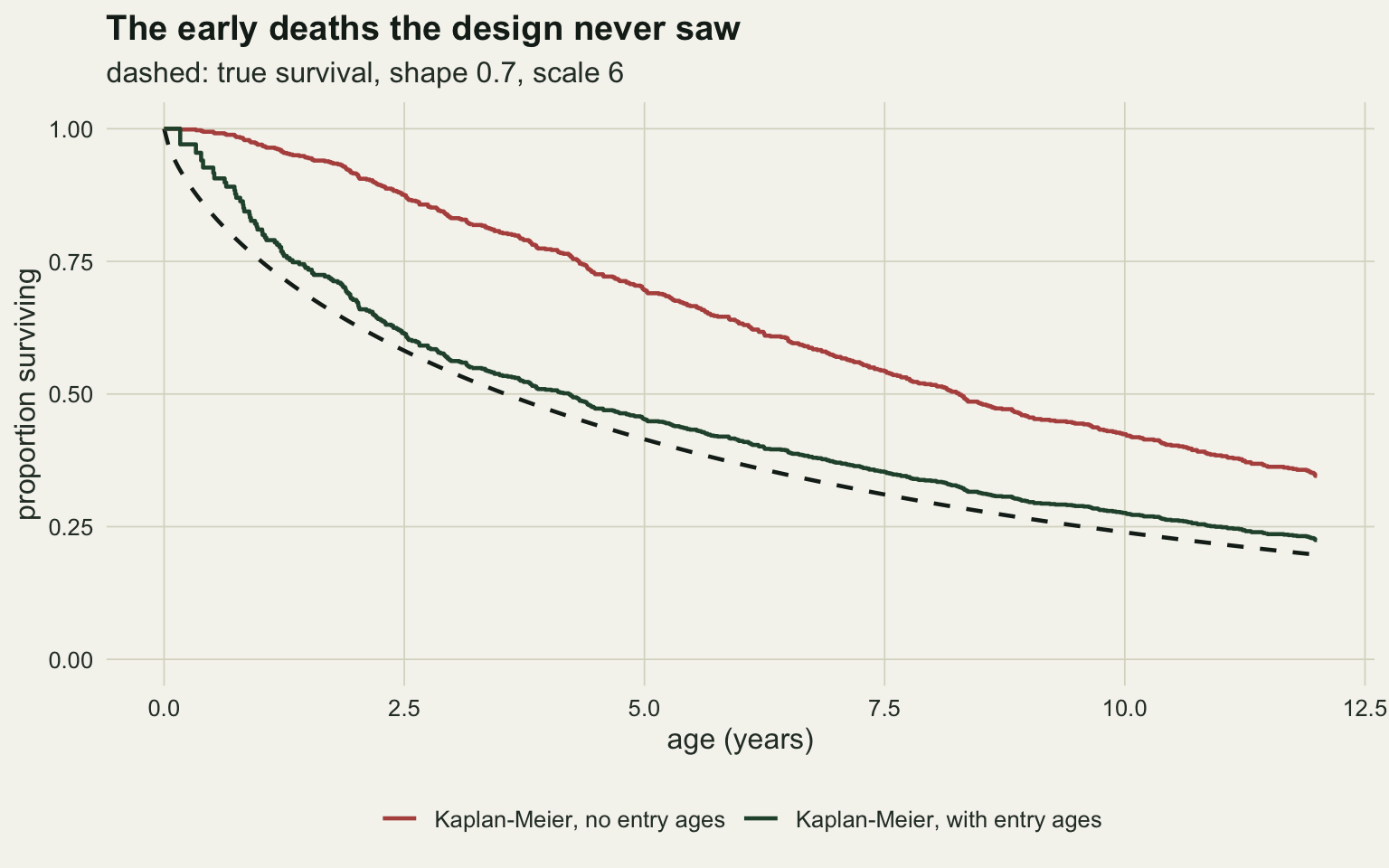

Figure 4: Kaplan-Meier survival for the worked data set, true shape 0.7 and marking ages up to 5 years, without and with the entry ages, against the true Weibull survival curve.

The curve with entry ages follows the truth but sits a little above it. Its first death is at age 0.17, when only 34 animals were at risk, and the true survival curve has already lost 0.078 of the population by then. So few animals were at risk at those ages that the curve missed those early deaths, and because every later value of a Kaplan-Meier curve is a product that includes that first stretch, the whole curve carries the missed step and sits above the truth. The curve without entry ages is far above the truth from the first year on, and it would read as a population with low mortality early in life.

How precise the repair is

The truncated likelihood removes the bias, but it does so from less information. An animal marked at age four says nothing about the risk of dying at age two, so the youngest ages are estimated from the few animals marked young, and the parameter that depends most on those ages pays for it.

tr_k_worst  <- grid_tab[which.max(abs(grid_tab$k_tr_pct)), ]
tr_m_worst  <- grid_tab[which.max(abs(grid_tab$m_tr_pct)), ]
m_tr_z      <- abs(grid_tab$m_tr_pct) / grid_tab$m_tr_se
k_tr_z      <- abs(grid_tab$k_tr_pct) / grid_tab$k_tr_se
n_cells     <- nrow(grid_tab)
sd_anchor   <- gcell(shape_anchor, entry_anchor)$m_tr_sd
sd_yearling <- gcell(shape_anchor, min(entry_set))$m_tr_sd
sd_widest   <- gcell(0.5, max(entry_set), n_small)$m_tr_sd

n_big <- 20000
n_big_rep <- 40
set.seed(9142)
big_runs <- t(replicate(n_big_rep, {
  dat <- sim_marked(n_big, tr_m_worst$shape, tr_m_worst$entry_max)
  f_tr <- fit_weib(dat, 1)
  c(k = f_tr[1], med = wb_median(f_tr[1], f_tr[2]))
}))
colnames(big_runs) <- c("k", "med")
big_med_pct <- 100 * (big_runs[, "med"] / wb_median(tr_m_worst$shape, wb_scale) - 1)
big_k_pct   <- 100 * (big_runs[, "k"] / tr_m_worst$shape - 1)
big_med_mean <- mean(big_med_pct); big_med_se <- sd(big_med_pct) / sqrt(n_big_rep)
big_k_mean   <- mean(big_k_pct);   big_k_se   <- sd(big_k_pct) / sqrt(n_big_rep)

Across all 48 cells, the largest error of the truncated shape is 2.2 per cent, at true shape 1.0, entry window 8.0 years and 200 animals, and the largest in Monte Carlo standard errors of a median is 2.1. The median lifespan is harder. Its largest error is 4.2 per cent, at true shape 0.5, entry window 8.0 years and 700 animals, and the largest in Monte Carlo standard errors is 2.2, which is about what the largest of 48 values of pure noise would reach. The standard error here is the normal approximation, 1.2533 times the standard deviation over the square root of the number of data sets.

To check that the median-lifespan error in that worst cell is noise and not a fault in the likelihood, the same design was run 40 times with 20000 animals. The mean error of the truncated median lifespan is +0.42 per cent with a standard error of 1.21, and the mean error of the shape +0.00 per cent with a standard error of 0.46.

The spread is the practical point. The standard deviation of the truncated median lifespan across data sets, as a share of the true median, is 8.2 per cent at true shape 0.7 with marking before half a year, 15.4 per cent with marking up to five years, and 61.2 per cent at true shape 0.5, marking up to eight years and 200 animals. The repair puts the estimate in the right place and reports honestly how little the design knows about the young.

When the entry age is only a minimum

The repair needs an entry age for every animal, and many studies do not have one. A lizard caught as a hatchling has a known age; one caught as an adult is often known only to be at least a year old, and a common coding puts such an animal in at its minimum age, entry at one year and death at one year plus the time since marking. That gives every animal an entry column, and the truncated likelihood above runs without complaint. It is not the same thing. Coding every adult at one fits the Weibull to time since marking, a mixture of the remaining lifetimes of animals marked at different true ages. Under a rising hazard an old animal has little life left and a young one a lot, and a Weibull fitted to that mixture has a flatter shape. It is the selection mechanism of census interval bias in tree mortality rates, with the age at marking as the unrecorded difference between animals. At a true shape of one the coding does no harm, because under a constant hazard the time an animal has left does not depend on its age.

The chunk keeps the generator above with one change: each animal is followed for a window of 4 to 10 years after marking, drawn uniformly and independently of its age, instead of to age 12, because censoring at a true age would tell the analysis that age. Marking ages run up to 2, 5 or 8 years, the true shapes are 1.6, 2.2 and 3.0, and each cell has 700 animals and 100 data sets, all fixed before the run. Animals marked before age one are juveniles of known age; the rest are adults whose age is unknown. Four fits are compared: the truncated likelihood with the true entry ages (a reference that a study marking adults would not have), minimum-age coding, the truncated likelihood on the juveniles alone, and an integrated likelihood that treats each adult’s age at marking as unknown between one year and the top of the marking window A. Marking at uniform ages among the living makes that age’s density proportional to the survival function S(a) on the interval, so an adult that dies t years after marking contributes S(1 + t) - S(A + t), and one still alive at the end of its window contributes the integral of S(a + t) over a from 1 to A, each divided by the integral of S from 1 to A; for a Weibull these integrals are incomplete gamma functions. This is the idea behind treating unknown birth years as latent, as Colchero and Clark (2012) do inside a capture-recapture model and the BaSTA package (Colchero, Jones and Rebke 2012) implements, written here for perfect detection and a known marking-age distribution.

fu_lo <- 4
fu_hi <- 10
n_rep_min <- 100
shape_min <- c(1.6, 2.2, 3.0)
entry_min <- c(2, 5, 8)

# marked animals followed for a window of calendar years, not to a fixed age
sim_window <- function(n_animals, shape, entry_max, skew = FALSE) {
  life <- entry <- numeric(0)
  while (length(life) < n_animals) {
    n_cand <- 3 * n_animals
    e_cand <- if (skew) entry_max * rbeta(n_cand, 1, 3) else runif(n_cand, 0, entry_max)
    l_cand <- rweibull(n_cand, shape, wb_scale)
    alive  <- l_cand > e_cand
    life   <- c(life, l_cand[alive])
    entry  <- c(entry, e_cand[alive])
  }
  life   <- life[seq_len(n_animals)]
  entry  <- entry[seq_len(n_animals)]
  follow <- runif(n_animals, fu_lo, fu_hi)
  list(entry = entry, time = pmin(life - entry, follow),
       dead = as.numeric(life - entry <= follow))
}

# integral of the Weibull survival function from lo to hi
int_surv <- function(lo, hi, k, s) {
  s / k * gamma(1 / k) * (pgamma((lo / s)^k, 1 / k, lower.tail = FALSE) -
                            pgamma((hi / s)^k, 1 / k, lower.tail = FALSE))
}
# adults of unknown age a in [1, a_max], marked with probability proportional to S(a)
nll_integ <- function(par, juv, adult, a_max) {
  k <- exp(par[1]); s <- exp(par[2])
  num <- ifelse(adult$dead == 1,
                pweibull(1 + adult$time, k, s, lower.tail = FALSE) -
                  pweibull(a_max + adult$time, k, s, lower.tail = FALSE),
                int_surv(1 + adult$time, a_max + adult$time, k, s))
  v <- nll_weib(par, juv$age, juv$dead, juv$entry, 1) -
    sum(log(num)) + length(num) * log(int_surv(1, a_max, k, s))
  if (is.finite(v)) v else 1e10
}

fit_codings <- function(dat, a_max) {
  juv <- dat$entry < 1
  e_min <- ifelse(juv, dat$entry, 1)
  known <- list(age = dat$entry + dat$time, dead = dat$dead, entry = dat$entry)
  minim <- list(age = e_min + dat$time, dead = dat$dead, entry = e_min)
  young <- lapply(known, function(v) v[juv])
  adult <- list(time = dat$time[!juv], dead = dat$dead[!juv])
  f_young <- fit_weib(young, 1)
  f_int <- optim(log(f_young), nll_integ, juv = young, adult = adult, a_max = a_max)
  c(known = fit_weib(known, 1)[1], minimum = fit_weib(minim, 1)[1],
    juveniles = f_young[1], integrated = exp(f_int$par[1]), n_juv = sum(juv))
}

set.seed(6604)
min_cells <- expand.grid(shape = shape_min, entry_max = entry_min)
min_runs <- lapply(seq_len(nrow(min_cells)), function(i) {
  t(replicate(n_rep_min, fit_codings(
    sim_window(n_keep, min_cells$shape[i], min_cells$entry_max[i]),
    min_cells$entry_max[i])))
})
med_of <- function(col) sapply(min_runs, function(r) median(r[, col]))
sd_of  <- function(col) sapply(min_runs, function(r) sd(r[, col]))
min_tab <- data.frame(min_cells,
                      known = med_of("known"), minimum = med_of("minimum"),
                      juveniles = med_of("juveniles"), integrated = med_of("integrated"),
                      sd_known = sd_of("known"), sd_juv = sd_of("juveniles"),
                      sd_int = sd_of("integrated"), n_juv = med_of("n_juv"),
                      min_lowest = sapply(min_runs, function(r) min(r[, "minimum"])))
# the value the minimum-age fit converges to: one very large data set per cell
min_limit <- sapply(seq_len(nrow(min_cells)), function(i) {
  big <- sim_window(1e5, min_cells$shape[i], min_cells$entry_max[i])
  e_min <- ifelse(big$entry < 1, big$entry, 1)
  fit_weib(list(age = e_min + big$time, dead = big$dead, entry = e_min), 1)[1]
})
# young-skewed marking effort, integrated fit still assuming uniform marking on [0, 8]
skew_runs <- t(replicate(n_rep_min, fit_codings(sim_window(n_keep, 3, 8, skew = TRUE), 8)))
skew_med  <- apply(skew_runs, 2, median)
mcell <- function(sh, em) min_tab[min_tab$shape == sh & min_tab$entry_max == em, ]
lim_of <- function(sh, em) min_limit[min_tab$shape == sh & min_tab$entry_max == em]
se_med <- function(sd_v) 1.2533 * sd_v / sqrt(n_rep_min)
juv_err <- max(abs(min_tab$juveniles - min_tab$shape))
juv_z   <- max(abs(min_tab$juveniles - min_tab$shape) / se_med(min_tab$sd_juv))
int_err <- max(abs(min_tab$integrated - min_tab$shape))
int_z   <- max(abs(min_tab$integrated - min_tab$shape) / se_med(min_tab$sd_int))
limit_gap <- max(abs(min_tab$minimum - min_limit))
skew_se <- se_med(sd(skew_runs[, "integrated"]))
# a weakly rising hazard outside the grid: minimum-age fits only, marking up to 8 years
min_fit <- function(d) { e <- ifelse(d$entry < 1, d$entry, 1)
  fit_weib(list(age = e + d$time, dead = d$dead, entry = e), 1)[1] }
weak_min   <- replicate(n_rep_min, min_fit(sim_window(n_keep, 1.2, 8)))
weak_limit <- min_fit(sim_window(1e5, 1.2, 8))

show_min <- data.frame(min_tab[, c("shape", "entry_max", "known", "minimum")],
                       limit = min_limit, min_tab[, c("juveniles", "integrated")])
names(show_min) <- c("true shape", "marking ages up to", "known age",
                     "minimum age", "minimum age, large-sample value",
                     "juveniles only", "integrated")
knitr::kable(show_min, digits = c(1, 0, 3, 3, 3, 3, 3), row.names = FALSE)

true shape	marking ages up to	known age	minimum age	minimum age, large-sample value	juveniles only	integrated
1.6	2	1.605	1.575	1.573	1.610	1.605
2.2	2	2.212	2.142	2.132	2.219	2.213
3.0	2	2.987	2.843	2.856	2.991	2.994
1.6	5	1.596	1.464	1.460	1.602	1.604
2.2	5	2.184	1.820	1.816	2.167	2.193
3.0	5	3.015	2.194	2.182	2.940	2.998
1.6	8	1.590	1.390	1.398	1.582	1.591
2.2	8	2.200	1.661	1.660	2.199	2.211
3.0	8	3.013	1.878	1.886	2.975	3.012

With the true entry ages the median shape is within 0.016 of the truth in every cell. Minimum-age coding flattens the hazard, by an amount set by the spread of marking ages. With marking up to 8 years, true shapes of 1.6, 2.2 and 3.0 read 1.390, 1.661 and 1.878; up to 5 years, 1.464, 1.820 and 2.194; up to 2 years, where a median of 353 of the 700 animals at true shape 3.0 are juveniles of known age, 1.575, 2.142 and 2.843. In this grid (true shapes 1.6 to 3.0) the flattening does not take the shape below one: the lowest single minimum-age estimate in all 900 data sets is 1.229, so a rising hazard still reads as rising, only less steeply. A weakly rising one can cross in a single data set: at a true shape of 1.2 with marking up to 8 years, run outside the grid with minimum-age fits only, the fit converges to 1.143 (one data set of 100 000 animals), still above one, but 1 of 100 data sets of 700 animals gave a shape below one. The two shortcuts err in opposite directions: leaving out the entry column steepened a rising hazard in the sections above, and coding adults at their minimum age flattens it.

The minimum-age number is not sampling noise. One data set of 100 000 animals per cell gives 1.398, 1.660 and 1.886 at the widest window, and the medians of the 700-animal fits are within 0.013 of these large-sample values in every cell. It is the value the fit converges to for a given design, fixed by the marking-age distribution and the true hazard, and a larger study only measures it more precisely.

Both repairs recover the shape. The juveniles alone give medians within 0.060 of the truth and the integrated likelihood within 0.013, at most 1.9 and 1.2 Monte Carlo standard errors of a median away. They differ in what they cost. At true shape 3.0 with marking up to 8 years, where a median of 133 animals are juveniles, the standard deviation of the shape across data sets is 0.115 with the true ages, 0.190 from the integrated likelihood and 0.262 from the juveniles alone. The integrated likelihood buys its precision with an assumption about who got marked. When marking effort favours young animals (marking ages drawn as 8 times a beta(1, 3) variable) and the fit still assumes uniform marking up to 8 years, its median at a true 3.0 is 2.966, 1.1 per cent below it, with a Monte Carlo standard error of 0.018, so this one wrong assumption cost little; minimum-age coding gives 2.391 and the juveniles alone 3.036 on the same data sets.

What to report

Record the age at entry for every animal, in the same row as its age at death or last sighting, and fit a likelihood that uses it. In R that is the three-column Surv(entry, age, dead) object for Kaplan-Meier curves and Cox models, a hand-coded likelihood like the one above for a Weibull, or flexsurv::flexsurvreg, whose documentation lists the same three-column Surv object among the responses it accepts for parametric models (it was not installed here, so it is not demonstrated in this post). Say in the methods that the fit is left-truncated at the marking age, because a reader cannot tell from a shape estimate whether it was.

Give the distribution of entry ages, at least its range and median, next to any hazard shape. The sweep above shows that the damage depends on the spread of entry ages and on the true shape together, and a reader can only judge the first from what the paper prints.

Before reading a Weibull shape as evidence of senescence, draw the Weibull plot from the Nelson-Aalen curve with the entry ages. A shape above one that is not there with the entry ages is not senescence. For a longitudinal design, Nussey and colleagues (2008) set out what else can make an age pattern in wild animals appear or disappear, and selective disappearance of frail individuals is among them.

If the entry ages were not kept, say so, and do not report the shape at all. The median lifespan is also inflated, and without the entry column there is no way to say by how much. An adult coded at its minimum age has no entry age either: fit the animals of known age alone, or integrate over the unknown age under a stated distribution of ages at marking, and say which.

Honest limits

Everything is a Weibull: the generating model and every fit. A real survival curve with a falling hazard early and a rising one late, which is the bathtub shape of many vertebrates, has no single Weibull shape to recover, and what the naive fit does to such a curve was not run. The truncated likelihood is correct for any parametric family, but only the Weibull was run.

Outside the section on minimum ages, age is known exactly. Skeletochronology, tooth wear and plumage all carry ageing error, and an error in the entry age enters the repair term directly. That section ran one form of it, adults known only to be older than one year, with perfect detection and the marking-age distribution assumed known, plus one case in which that assumption was wrong; an age that is estimated with error rather than bounded was not run, and in a capture-recapture study the latent-age likelihood also needs the detection model that Colchero and Clark (2012) build in.

Entry ages are uniform over a window (apart from the one young-skewed case in the section on minimum ages) and independent of the animal’s lifetime. If marking effort is higher at some ages than others the truncation changes shape, and if the chance of being caught depends on the animal’s condition, the marked animals differ from their cohort in more than age. Detection is perfect after marking: every retained animal is followed to death or to age 12 (in the section on minimum ages, to death or to the end of a follow-up window of 4 to 10 years after marking). In a mark-recapture study, deaths are not observed directly and the likelihood needs a detection model on top of the truncation.

The grid has one scale, one censoring age and two sample sizes; the section on minimum ages used a follow-up window instead of the censoring age, and one sample size. The discard share, and with it the damage, depends on how far the entry window reaches into the lifetime distribution, so the per cent figures above belong to a scale of six years and a window of up to eight; what transfers is the direction, the ordering by true shape and by entry spread, and the one-term repair.

References

Klein JP, Moeschberger ML 2003 Survival Analysis: Techniques for Censored and Truncated Data, 2nd edn (ISBN 978-0-387-95399-1)

Kalbfleisch JD, Prentice RL 2002 The Statistical Analysis of Failure Time Data, 2nd edn (ISBN 978-0-471-36357-6)

Colchero F, Clark JS 2012 Journal of Animal Ecology 81(1):139-149 (10.1111/j.1365-2656.2011.01898.x)

Colchero F, Jones OR, Rebke M 2012 Methods in Ecology and Evolution 3(3):466-470 (10.1111/j.2041-210X.2012.00186.x)

Nussey DH, Coulson T, Festa-Bianchet M, Gaillard JM 2008 Functional Ecology 22(3):393-406 (10.1111/j.1365-2435.2008.01408.x)

Related tutorials

• Interval-censored survival from visit data
• Lost collar signals and informative censoring
• Fitting a senescence model to individual records
• Time-varying covariates in a survival model