library(survival)
library(ggplot2)

te_paper  <- "#f5f4ee"
te_ink    <- "#16241d"
te_body   <- "#2c3a31"
te_forest <- "#275139"
te_rust   <- "#b5534e"
te_gold   <- "#c9b458"
te_line   <- "#dad9ca"

theme_datasheet <- function() {
  theme_minimal(base_size = 12) +
    theme(plot.background  = element_rect(fill = te_paper, colour = NA),
          panel.background = element_rect(fill = te_paper, colour = NA),
          panel.grid.major = element_line(colour = te_line, linewidth = 0.3),
          panel.grid.minor = element_blank(),
          text             = element_text(colour = te_body),
          plot.title       = element_text(colour = te_ink, face = "bold"),
          plot.subtitle    = element_text(colour = te_body),
          axis.text        = element_text(colour = te_body),
          strip.text       = element_text(colour = te_ink, face = "bold"))
}Lost collar signals and informative censoring
R
survival analysis
telemetry
censoring
simulation
ecology tutorial
When dead animals silence their collars, Kaplan-Meier survival runs high. Testing in R how far a battery-life likelihood and a cut-off rule can be trusted.
A wolf study puts GPS collars on 120 animals and follows them for two years. Some collars send a mortality signal and a crew walks in to find the carcass. Many more simply go quiet. A battery at the end of its life goes quiet, but so does a collar that was cut off by a poacher, crushed by a vehicle, or left on a carcass in a snow hole where the signal never reaches the satellite. In the data sheet both kinds of silence end up in the same column, “signal lost”, and the standard analysis censors them.
The site’s post on Kaplan-Meier survival curves sets up exactly that data. Its simulation draws the censoring times with rexp() and the comment # collar failure or emigration, independent of the death times, which is the assumption under which censoring is harmless. The post on competing risks and cumulative incidence has two causes of death, but both are observed: every animal that dies is known to have died, and of which cause. The post on missing data mechanisms gives “A logger battery that fails on a random schedule” as its example of data missing completely at random, and fits no survival model. This post drops the independence assumption. A share q of deaths is recorded as a lost signal, and the question is what can be done about it.
None of the concern is new. Pollock and colleagues set out the Kaplan-Meier estimator with staggered entry for telemetry in 1989 and listed censoring unrelated to fate among its assumptions; Tsai, Pollock and Brownie examined by simulation what violated assumptions do to these estimators; Murray reviewed telemetry survival estimation in 2006 with the same caution; and Heisey and Patterson framed the fates of collared animals as competing risks. The upward bias of Kaplan-Meier is a closed form and is shown here only as the starting line. What the post measures are two repairs a field analyst might reach for: a likelihood that separates hidden deaths from battery failures by leaning on the bench battery-life curve, and a field rule, used here as an illustrative convention, that calls every loss before 60 per cent of nominal battery life a death. Both depend on a battery number nobody knows exactly, and the measurement is how much each one suffers when that number is off.
A collar study with two kinds of silence
Deaths follow a seasonal hazard: a winter rate from day 300 to day 90 of each year and a lower summer rate in between, so the true one-year survival is known exactly. Collar batteries fail on a Weibull wear-out curve with a steep shape, and the Weibull scale is called the nominal life here: the day by which 63 per cent of collars have died. When an animal dies before its battery does, the death is seen with probability 1 - q and becomes a lost signal with probability q. The study ends at day 730. Every constant below was set before any estimator was run, and none was changed afterwards.
t_end   <- 730                      # administrative end of the study, days
hz_win  <- 0.0022                   # daily death hazard, winter
hz_sum  <- 0.0006                   # daily death hazard, summer
bat_shp <- 5                        # Weibull shape of collar battery life
bat_scl <- 520                      # Weibull scale, the nominal life in days
cut_frac <- 0.6                     # field rule: losses before this share of nominal life
n_animal <- 120                     # collared animals per study
n_rep    <- 400                     # simulated studies per cell

is_winter <- function(d) { r <- d %% 365; r < 90 | r >= 300 }
day_mid <- seq_len(t_end) - 0.5
cum_win <- c(0, cumsum(is_winter(day_mid)))
cum_haz <- c(0, cumsum(ifelse(is_winter(day_mid), hz_win, hz_sum)))
win_365 <- cum_win[366]
S1_true <- exp(-cum_haz[366])       # true one-year survival

winter_days <- function(tt) {
  f <- pmin(floor(tt), t_end - 1)
  cum_win[f + 1] + (tt - f) * is_winter(f + 0.5)
}

sim_study <- function(n, q, shp = bat_shp, scl = bat_scl, p_early = 0, early_mean = 60) {
  u  <- rexp(n)
  td <- approx(cum_haz, 0:t_end, xout = u, rule = 2, ties = "ordered")$y
  td[u >= max(cum_haz)] <- Inf
  tb <- rweibull(n, shp, scl)
  if (p_early > 0) {
    early <- runif(n) < p_early
    tb[early] <- pmin(tb[early], rexp(sum(early), 1 / early_mean))
  }
  tt <- pmin(td, tb, t_end)
  fate <- ifelse(tt == t_end, "end",
          ifelse(td < tb, ifelse(runif(n) < q, "lost", "dead"), "lost"))
  list(t = tt, fate = fate, tb = tb, hidden = td < tb & fate == "lost")
}
Four estimators of one-year survival are compared. Kaplan-Meier with every loss censored is the default. Kaplan-Meier with every loss counted as a death is the pessimistic bound; it is still an estimator of something, but it books every battery failure as a death. The cut-off rule counts a loss as a death if it happens before 60 per cent of the nominal life and censors it otherwise. The likelihood treats a lost signal as the outcome of two hazards acting together: q times the death hazard, plus the battery hazard taken from the bench curve. Deaths contribute (1 - q) times the death hazard, and everyone contributes the survival term of the death process; the battery survival term does not depend on the parameters and drops out. The two seasonal rates and q are estimated, and the battery curve is plugged in. For speed the Kaplan-Meier value at day 365 is computed by hand, with a log-log Greenwood interval, and checked once against survfit().
km_at <- function(tt, ev, at = 365) {
  o <- order(tt, -ev); tt <- tt[o]; ev <- ev[o]
  at_risk <- length(tt) - seq_along(tt) + 1
  k <- ev & tt <= at
  ut <- unique(tt[k])
  if (!length(ut)) return(c(S = 1, lo = 1, hi = 1))
  d_n <- tabulate(match(tt[k], ut), length(ut)); r_n <- at_risk[match(ut, tt)]
  S <- prod(1 - d_n / r_n); v <- sum(d_n / (r_n * (r_n - d_n)))
  if (S <= 0 || S >= 1) return(c(S = S, lo = S, hi = S))
  se <- sqrt(v) / abs(log(S)); lS <- log(-log(S))
  c(S = S, lo = exp(-exp(lS + 1.96 * se)), hi = exp(-exp(lS - 1.96 * se)))
}

nll_cr <- function(p, W, U, dd, ll, wi, hb) {
  hw <- exp(p[1]); hs <- exp(p[2]); q <- plogis(p[3])
  h <- ifelse(wi, hw, hs); den <- q * h + hb
  -(-sum(W) * hw - sum(U) * hs + sum(dd) * log(1 - q) + sum(log(h[dd])) + sum(log(den[ll])))
}
grad_cr <- function(p, W, U, dd, ll, wi, hb) {
  hw <- exp(p[1]); hs <- exp(p[2]); q <- plogis(p[3])
  h <- ifelse(wi, hw, hs); den <- q * h + hb
  -c(-sum(W) * hw + sum(dd & wi) + sum((q * h * wi / den)[ll]),
     -sum(U) * hs + sum(dd & !wi) + sum((q * h * (!wi) / den)[ll]),
     -q * sum(dd) + sum((h * q * (1 - q) / den)[ll]))
}
fit_cr <- function(D, shp, scl, ci = FALSE) {
  W <- winter_days(D$t); U <- D$t - W; wi <- is_winter(D$t)
  dd <- D$fate == "dead"; ll <- D$fate == "lost"
  hb <- (shp / scl) * (D$t / scl)^(shp - 1)          # bench battery hazard
  o <- optim(c(log(0.001), log(0.001), 0), nll_cr, grad_cr, W = W, U = U,
             dd = dd, ll = ll, wi = wi, hb = hb, method = "BFGS")
  H1 <- win_365 * exp(o$par[1]) + (365 - win_365) * exp(o$par[2])
  out <- c(S = exp(-H1), q = plogis(o$par[3]), conv = o$convergence, lo = NA, hi = NA)
  if (ci) {
    hess <- optimHess(o$par, nll_cr, grad_cr, W = W, U = U, dd = dd, ll = ll, wi = wi, hb = hb)
    vc <- tryCatch(solve(hess), error = function(e) matrix(NA, 3, 3))
    g <- c(win_365 * exp(o$par[1]), (365 - win_365) * exp(o$par[2]), 0) / H1
    se <- sqrt(drop(t(g) %*% vc %*% g))
    out[c("lo", "hi")] <- exp(-H1 * exp(c(1.96, -1.96) * se))
  }
  out
}
rule_S <- function(D, nominal, frac = cut_frac)
km_at(D$t, D$fate == "dead" | (D$fate == "lost" & D$t < frac * nominal))set.seed(4120)
D1 <- sim_study(n_animal, q = 0.3)
n_dead <- sum(D1$fate == "dead"); n_lost <- sum(D1$fate == "lost")
n_hidden <- sum(D1$hidden); n_batt <- n_lost - n_hidden; n_end <- sum(D1$fate == "end")
ex_km <- km_at(D1$t, D1$fate == "dead")
sv <- summary(survfit(Surv(D1$t, D1$fate == "dead") ~ 1, conf.type = "log-log"), times = 365)
km_gap <- max(abs(ex_km - c(sv$surv, sv$lower, sv$upper)))
ex_bound <- km_at(D1$t, D1$fate != "end")[["S"]]
ex_rule <- rule_S(D1, bat_scl)[["S"]]
ex_mle <- fit_cr(D1, bat_shp, bat_scl, ci = TRUE)In this one study of 120 animals the crew found 30 carcasses and lost 90 signals, and 0 collars were still working on a live animal at day 730. Of the lost signals 20 were deaths and 70 were batteries, a split nobody in the field would know. The hand-written Kaplan-Meier matches survfit() to 1.9e-06 in the estimate and both interval ends.
True one-year survival is 0.627. Censoring the losses gives 0.788, with an interval from 0.697 to 0.854 that misses the truth. Counting every loss as a death gives 0.550, the cut-off rule 0.649, and the likelihood with the correct battery curve 0.662 (interval 0.568 to 0.740), with q estimated at 0.40 against a design value of 0.3.
Kaplan-Meier rises to S to the power one minus q
If battery failures are independent of fate, censoring every loss removes exactly the hidden deaths from the death hazard. The recorded death hazard is (1 - q) times the true one, so Kaplan-Meier estimates S to the power 1 - q. That is arithmetic, and the simulation should reproduce it. The grid below runs 400 studies of 120 animals at each value of q, and inside every study it also fits the likelihood at seven bench curves and the cut-off rule at five cut-offs, so the next two sections read from the same simulated studies.
q_grid <- c(0, 0.1, 0.3, 0.5)
mult_grid <- c(0.7, 0.8, 0.9, 1, 1.1, 1.2, 1.3) # bench scale over true scale
frac_grid <- c(0.4, 0.5, 0.6, 0.7, 0.8)

one_study <- function(n, q, scl = bat_scl, mult = mult_grid, p_early = 0, fracs = frac_grid) {
  D <- sim_study(n, q, scl = scl, p_early = p_early)
  k <- km_at(D$t, D$fate == "dead")
  b <- km_at(D$t, D$fate != "end")
  r <- c(km = k[["S"]], km_cov = k[["lo"]] <= S1_true & S1_true <= k[["hi"]],
         bound = b[["S"]], bracket = b[["lo"]] <= S1_true & S1_true <= k[["hi"]],
         width = k[["hi"]] - b[["lo"]],
         q_real = sum(D$hidden) / max(1, sum(D$hidden | D$fate == "dead")))
  for (f in fracs) r[paste0("frac_", f)] <- rule_S(D, scl, f)[["S"]]
  for (m in mult) {
    z <- fit_cr(D, bat_shp, m * scl, ci = m == 1)
    r[paste0("S_", m)] <- z[["S"]]; r[paste0("q_", m)] <- z[["q"]]
    r[paste0("conv_", m)] <- z[["conv"]]
    r[paste0("rule_", m)] <- rule_S(D, m * scl)[["S"]]
    if (m == 1) r["mle_cov"] <- z[["lo"]] <= S1_true & S1_true <= z[["hi"]]
  }
  r
}
set.seed(20918)
t_grid <- system.time(
  grid_res <- lapply(q_grid, function(q) t(replicate(n_rep, one_study(n_animal, q))))
)[["elapsed"]]
names(grid_res) <- q_grid

rmse <- function(x) sqrt(mean((x - S1_true)^2))
mcse_rmse <- function(x) sd((x - S1_true)^2) / (2 * rmse(x) * sqrt(length(x)))
col_stat <- function(q, col, fun = mean) fun(grid_res[[as.character(q)]][, col])

km_tab <- data.frame(q = q_grid,
  km = sapply(q_grid, col_stat, col = "km"),
  closed = S1_true^(1 - q_grid),
  bound = sapply(q_grid, col_stat, col = "bound"),
  rule = sapply(q_grid, col_stat, col = "rule_1"),
  mle = sapply(q_grid, col_stat, col = "S_1"),
  km_cov = sapply(q_grid, col_stat, col = "km_cov"),
  mle_cov = sapply(q_grid, col_stat, col = "mle_cov"),
  q_hat = sapply(q_grid, col_stat, col = "q_1"),
  q_real = sapply(q_grid, col_stat, col = "q_real"))
km_formula_gap <- max(abs(km_tab$km - km_tab$closed))
max_mcse_mean <- max(sapply(q_grid, function(q) sapply(c("km", "S_1", "rule_1"),
  function(cc) sd(grid_res[[as.character(q)]][, cc]) / sqrt(n_rep))))
n_nonconv <- sum(sapply(grid_res, function(M) sum(M[, grep("^conv_", colnames(M))] != 0)))
round(km_tab, 3)
q km closed bound rule mle km_cov mle_cov q_hat q_real
1 0.0 0.627 0.627 0.531 0.580 0.627 0.940 0.952 0.002 0.000
2 0.1 0.660 0.657 0.531 0.590 0.627 0.908 0.950 0.101 0.100
3 0.3 0.720 0.721 0.529 0.602 0.627 0.483 0.945 0.292 0.297
4 0.5 0.790 0.792 0.530 0.615 0.628 0.068 0.940 0.493 0.496The closed form holds: across the four values of q, mean Kaplan-Meier and S to the power 1 - q differ by at most 0.003, against a Monte Carlo standard error of at most 0.0023 for any mean in the table. At q = 0.3 Kaplan-Meier averages 0.720 against the formula’s 0.721, and its nominal 95 per cent interval covers the truth in 48.3 per cent of studies; at q = 0.5 in 6.8 per cent.
The likelihood with the true battery curve averages between 0.627 and 0.628 at every q, its interval covers in 94.0 to 95.2 per cent of studies (Monte Carlo standard error 0.011), and its estimate of q at 0.3 averages 0.292. Of the 11200 likelihood fits in the grid, 0 failed to converge. The cut-off rule sits below the truth at every q, from 0.580 at q = 0 to 0.615 at q = 0.5: batteries that die before the cut-off are booked as deaths, and hidden deaths after it are censored, and in this design the first error is the larger.
km_long <- rbind(
  data.frame(q = q_grid, est = km_tab$km, method = "Kaplan-Meier, losses censored"),
  data.frame(q = q_grid, est = km_tab$bound, method = "all losses as deaths"),
  data.frame(q = q_grid, est = km_tab$rule, method = "60 per cent rule"),
  data.frame(q = q_grid, est = km_tab$mle, method = "likelihood, true battery curve"))
km_long$method <- factor(km_long$method, levels = unique(km_long$method))
q_fine <- seq(0, 0.5, by = 0.01)
ggplot(km_long, aes(q, est, colour = method)) +
  geom_hline(yintercept = S1_true, colour = te_body, linetype = "dashed", linewidth = 0.5) +
  geom_line(data = data.frame(q = q_fine, est = S1_true^(1 - q_fine)),
            aes(q, est), inherit.aes = FALSE, colour = te_ink, linetype = "dotted", linewidth = 0.7) +
  geom_line(linewidth = 0.9) + geom_point(size = 2.4) +
  scale_colour_manual(values = c(te_rust, te_ink, te_gold, te_forest), name = NULL) +
  guides(colour = guide_legend(nrow = 2)) +
  labs(x = "share of deaths that silence the collar (q)", y = "mean estimated one-year survival",
       title = "Hidden deaths lift Kaplan-Meier along a closed form",
       subtitle = "dashed: true survival; dotted: S^(1 - q)") +
  theme_datasheet() + theme(legend.position = "bottom")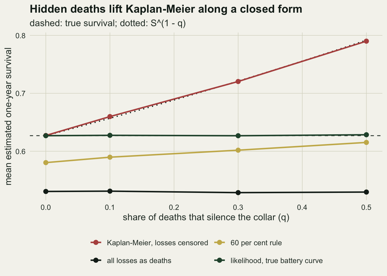
The all-losses-as-deaths bound does not move with q, because every death is counted either way; its level, 0.529 at q = 0.3, is set by how many batteries fail inside the first year. Between them the two Kaplan-Meier versions bracket the truth whatever q is, and that bracket comes back below.
A bench curve that is slightly wrong
The likelihood needs the battery hazard at every loss time. In practice that curve comes from the manufacturer or from bench tests, and a bench is not a cold winter on a moving animal with a fix schedule that changes by season. The grid fitted every study with the bench scale set from 0.7 to 1.3 times the true one, the shape held at its true value. To be fair to the rule, the rule also takes its nominal life from the same bench number: a field crew applying “60 per cent of nominal life” has nothing else to apply it to.
bench_long <- do.call(rbind, lapply(q_grid, function(q) {
  M <- grid_res[[as.character(q)]]
  rbind(data.frame(q = q, mult = mult_grid, method = "likelihood",
                   rmse = sapply(mult_grid, function(m) rmse(M[, paste0("S_", m)])),
                   mean = sapply(mult_grid, function(m) mean(M[, paste0("S_", m)]))),
        data.frame(q = q, mult = mult_grid, method = "60 per cent rule",
                   rmse = sapply(mult_grid, function(m) rmse(M[, paste0("rule_", m)])),
                   mean = sapply(mult_grid, function(m) mean(M[, paste0("rule_", m)]))))
}))
km_rmse <- sapply(q_grid, function(q) rmse(grid_res[[as.character(q)]][, "km"]))
names(km_rmse) <- q_grid
bget <- function(q, m, meth, what = "rmse")
  bench_long[[what]][bench_long$q == q & bench_long$mult == m & bench_long$method == meth]
# first optimistic bench multiplier at which the likelihood loses to plain Kaplan-Meier
break_even <- sapply(q_grid, function(q) {
  up <- mult_grid[mult_grid > 1]
  worse <- up[sapply(up, function(m) bget(q, m, "likelihood") > km_rmse[[as.character(q)]])]
  if (length(worse)) min(worse) else NA
})
names(break_even) <- q_grid
max_mcse_rmse <- max(sapply(q_grid, function(q) sapply(mult_grid, function(m)
  mcse_rmse(grid_res[[as.character(q)]][, paste0("S_", m)]))))
q3 <- grid_res[["0.3"]]
q_hat_lo <- mean(q3[, "q_0.7"]); q_hat_hi <- mean(q3[, "q_1.3"])
rule_bound_mult <- 365 / (cut_frac * bat_scl)
bracket_q <- sapply(q_grid, col_stat, col = "bracket")
width_q <- sapply(q_grid, col_stat, col = "width")
A bench life that is too long is an optimistic curve. It says batteries should still be alive at the loss times, so the model hands more of the losses to death: at q = 0.3 the estimate of q averages 0.494 at 1.3 times the true life and 0.161 at 0.7 times, and survival follows. At q = 0.3 the root mean square error of the likelihood is 0.064 at 0.7 and 0.114 at 1.3, and at 0.8 and 1.2 it is 0.058 and 0.085. The Monte Carlo standard error of any of these errors is below 0.0020.
km_ref <- data.frame(q = q_grid, rmse = km_rmse)
lab_q <- function(x) paste("q =", x)
ggplot(bench_long, aes(mult, rmse, colour = method)) +
  geom_hline(data = km_ref, aes(yintercept = rmse), colour = te_rust,
             linetype = "dashed", linewidth = 0.6) +
  geom_vline(xintercept = 1, colour = te_line, linewidth = 0.6) +
  geom_line(linewidth = 0.9) + geom_point(size = 2) +
  facet_wrap(~ q, nrow = 1, labeller = as_labeller(lab_q)) +
  scale_colour_manual(values = c(likelihood = te_forest, "60 per cent rule" = te_gold), name = NULL) +
  scale_x_continuous(breaks = c(0.7, 1, 1.3)) +
  labs(x = "bench battery life relative to the true life", y = "RMSE of one-year survival",
       title = "An optimistic bench curve costs more than a pessimistic one",
       subtitle = "dashed red: Kaplan-Meier with losses censored") +
  theme_datasheet() + theme(legend.position = "bottom")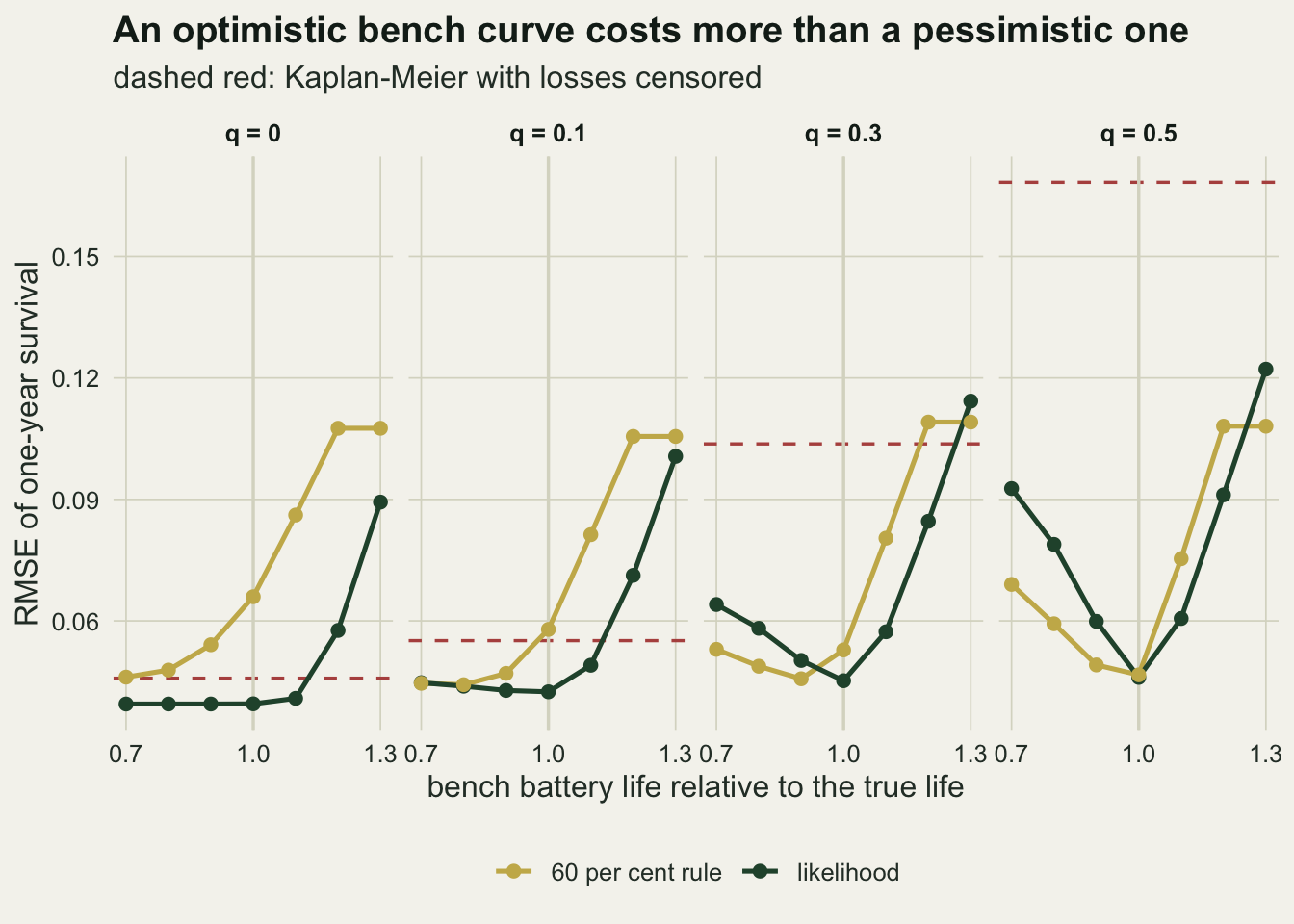
The dashed line is the reason anybody would bother. At q = 0.5 Kaplan-Meier is so far off (error 0.168) that the likelihood beats it at every bench curve in the grid. At q = 0.3 the likelihood first loses to doing nothing at 1.3 times the true life. At q = 0.1 it already loses at 1.2 times, and at q = 0 at 1.2 times, while at 1.1 times it is still ahead (0.049 against 0.055 at q = 0.1). The grid has no point between 1.1 and 1.2, so the break-even at low q lies somewhere in that step. On the pessimistic side the likelihood does not lose to Kaplan-Meier at any q in the grid; at q = 0, where there is nothing to repair, a short bench curve costs nothing at all because the estimate of q stays near zero.
The comparison with the rule does not favour the rule as a safer shortcut. With the true life the likelihood has the smaller error at q up to 0.3, from 0.040 against 0.066 at q = 0 to 0.045 against 0.053 at q = 0.3, and at q = 0.5 the two tie within Monte Carlo error (0.046 and 0.047). With a pessimistic bench number the rule is the steadier of the two once q is 0.3 or more: at 0.7 times the true life and q = 0.5 it scores 0.069 against the likelihood’s 0.093. With an optimistic one, at 1.1 and 1.2 times the true life, the rule is worse at every q; at 1.1 times and q = 0.3 it scores 0.080 against 0.057. Only at 1.3 times, where both have fallen to errors above 0.10 at q = 0.3, does the rule edge back ahead, at q = 0.3 and q = 0.5. The rule is not less fragile. It is less fragile to a pessimistic battery number and more fragile to an optimistic one, and the optimistic side is the one where the likelihood also fails.
The cut-off rule leans on the same number
The rule has a second number in it, the 60 per cent, and a second failure. Once 60 per cent of the nominal life reaches day 365, every loss in the first year is booked as a death and the rule at one year is the pessimistic bound. With a bench life 1.17 times the true one that has already happened, which is why its two right-most points in the previous figure lie on the same level. Holding the nominal life at its true value and moving the cut-off shows the other side.
frac_long <- do.call(rbind, lapply(q_grid, function(q) {
  M <- grid_res[[as.character(q)]]
  data.frame(q = factor(q), frac = frac_grid,
             mean = sapply(frac_grid, function(f) mean(M[, paste0("frac_", f)])))
}))
fget <- function(q, f) frac_long$mean[frac_long$q == q & frac_long$frac == f]
best_frac <- sapply(q_grid, function(q) {
  M <- grid_res[[as.character(q)]]
  frac_grid[which.min(sapply(frac_grid, function(f) rmse(M[, paste0("frac_", f)])))]
})
ggplot(frac_long, aes(frac, mean, colour = q)) +
  geom_hline(yintercept = S1_true, colour = te_body, linetype = "dashed", linewidth = 0.5) +
  geom_vline(xintercept = 365 / bat_scl, colour = te_body, linetype = "dotted", linewidth = 0.6) +
  geom_line(linewidth = 0.9) + geom_point(size = 2.2) +
  scale_colour_manual(values = c(te_ink, te_forest, te_gold, te_rust), name = "q") +
  labs(x = "cut-off as a share of nominal battery life", y = "mean estimated one-year survival",
       title = "The right cut-off depends on the unknown q",
       subtitle = "dashed: true survival; dotted: cut-off reaches day 365") +
  theme_datasheet() + theme(legend.position = "right")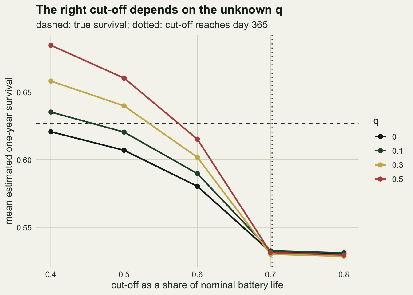
The cut-off with the smallest error in this grid is 0.4 of nominal life at q = 0, 0.5 at q = 0.1 and at q = 0.3, and 0.6 at q = 0.5 (at q = 0 the best value sits at the edge of the grid; with nothing to repair, the best cut-off is none at all). A rule tuned for one value of q is biased at another, and q is the unknown the rule was supposed to get around. At 0.7 of nominal life the cut-off falls on day 364, one day short of day 365, and at 0.8 it is past it, so at both every q gives the bound or next to it, about 0.53.
A short battery and an early failure mode
Two departures from the tidy set-up follow. In the first the battery wears out at a scale of 300 days, inside the first year, so hidden deaths and battery failures pile up in the same months. In the second, one collar in ten carries an electronic fault that kills it on an exponential clock with a mean of 60 days, on top of the wear-out curve; the bench curve used by the likelihood and the nominal life used by the rule still describe the wear-out alone. That second case is the question a wildlife biometrician asks first: field failures are not all wear-out, and an early failure looks like an early death.
scen <- list(list(lab = "baseline", q = 0.3, scl = bat_scl, pe = 0),
             list(lab = "wear-out at 300 d", q = 0.3, scl = 300, pe = 0),
             list(lab = "early failures, q = 0", q = 0, scl = bat_scl, pe = 0.1),
             list(lab = "early failures, q = 0.3", q = 0.3, scl = bat_scl, pe = 0.1))
set.seed(31702)
stress <- do.call(rbind, lapply(scen, function(s) {
  M <- t(replicate(n_rep, one_study(n_animal, s$q, scl = s$scl, mult = 1,
                                    p_early = s$pe, fracs = cut_frac)))
  cols <- c(km = "Kaplan-Meier", bound = "all losses as deaths",
            rule_1 = "60 per cent rule", S_1 = "likelihood, bench curve")
  data.frame(scenario = s$lab, method = unname(cols),
             mean = sapply(names(cols), function(cc) mean(M[, cc])),
             lo = sapply(names(cols), function(cc) quantile(M[, cc], 0.1)),
             hi = sapply(names(cols), function(cc) quantile(M[, cc], 0.9)),
             rmse = sapply(names(cols), function(cc) rmse(M[, cc])),
             mle_cov = mean(M[, "mle_cov"]), bracket = mean(M[, "bracket"]),
             width = mean(M[, "width"]))
}))
rownames(stress) <- NULL
sget <- function(sc, meth, what = "mean") stress[[what]][stress$scenario == sc & stress$method == meth]
p_early_batt <- 0.1 * (1 - exp(-365 / 60))
print(stress[, c("scenario", "method", "mean", "rmse")], digits = 3)
scenario method mean rmse
1 baseline Kaplan-Meier 0.7187 0.1026
2 baseline all losses as deaths 0.5273 0.1096
3 baseline 60 per cent rule 0.5982 0.0552
4 baseline likelihood, bench curve 0.6243 0.0454
5 wear-out at 300 d Kaplan-Meier 0.7205 0.1202
6 wear-out at 300 d all losses as deaths 0.0439 0.5833
7 wear-out at 300 d 60 per cent rule 0.6200 0.0698
8 wear-out at 300 d likelihood, bench curve 0.6326 0.0531
9 early failures, q = 0 Kaplan-Meier 0.6276 0.0475
10 early failures, q = 0 all losses as deaths 0.4769 0.1570
11 early failures, q = 0 60 per cent rule 0.5229 0.1133
12 early failures, q = 0 likelihood, bench curve 0.5375 0.0989
13 early failures, q = 0.3 Kaplan-Meier 0.7217 0.1055
14 early failures, q = 0.3 all losses as deaths 0.4802 0.1538
15 early failures, q = 0.3 60 per cent rule 0.5459 0.0927
16 early failures, q = 0.3 likelihood, bench curve 0.5475 0.0917With the short battery both repairs survive, as long as the bench curve is right: the likelihood averages 0.633 and the rule 0.620, with errors of 0.053 and 0.070. Counting every loss as a death collapses to 0.044, because nearly every collar is dead within the year.
The early failures break both. Before day 365 they remove about 10 per cent of collars, and neither repair has any way to tell them from hidden deaths. With no hidden deaths at all (q = 0) Kaplan-Meier is right, at 0.628, and the two repairs invent mortality: the rule gives 0.523, the likelihood 0.538, and the likelihood interval covers the truth in 39.5 per cent of studies. At q = 0.3 the two repairs land on 0.546 and 0.548, now nearly as far below the truth as Kaplan-Meier (0.722) is above it.
stress$scenario <- factor(stress$scenario, levels = rev(sapply(scen, `[[`, "lab")))
stress$method <- factor(stress$method, levels = c("Kaplan-Meier", "all losses as deaths",
                                                  "60 per cent rule", "likelihood, bench curve"))
ggplot(stress, aes(mean, scenario, colour = method)) +
  geom_vline(xintercept = S1_true, colour = te_body, linetype = "dashed", linewidth = 0.5) +
  geom_errorbar(aes(xmin = lo, xmax = hi), orientation = "y", width = 0.25,
                position = position_dodge(width = 0.7), linewidth = 0.5) +
  geom_point(size = 2.4, position = position_dodge(width = 0.7)) +
  scale_colour_manual(values = c(te_rust, te_ink, te_gold, te_forest), name = NULL) +
  guides(colour = guide_legend(nrow = 2)) +
  labs(x = "estimated one-year survival (mean, 10th to 90th percentile)", y = NULL,
       title = "Early collar failures look like deaths to both repairs",
       subtitle = "dashed: true survival") +
  theme_datasheet() + theme(legend.position = "bottom")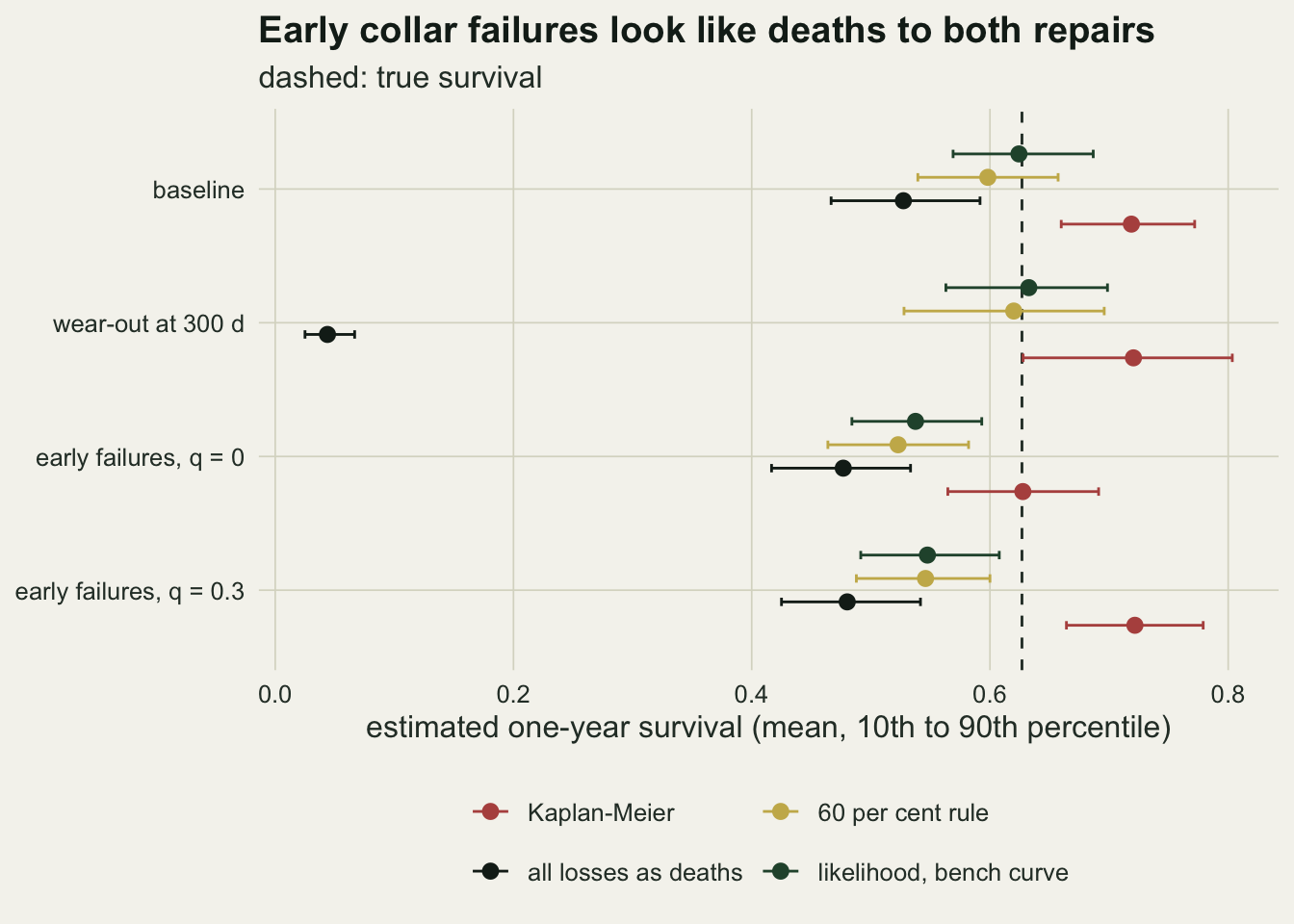
The bracket formed by the two Kaplan-Meier versions keeps covering the truth in all of this, because it does not use the battery curve. Taking the lower interval end of the all-losses-as-deaths version and the upper interval end of the losses-censored version, the bracket contained the truth in 100.0 per cent of studies with early failures at q = 0.3 and in 96.5 per cent at q = 0. The price is width: 0.41 on the survival scale in that scenario. With the 300-day battery the bracket holds too, in 100.0 per cent of studies, but its average width is 0.81: it covers because it spans most of the survival scale, and it says next to nothing about survival exactly when batteries die inside the year.
Retrieved collars as the battery curve
A study does not have to rely on the manufacturer. Collars come back working from animals found dead and, in longer-lived designs, from survivors at the end. If each is left running on the fix schedule until it dies, its total life is a battery lifetime observed without reference to the lost animals. Those lifetimes are not a random sample, though. A collar is only retrieved if it was still working on the day the animal was found, so short-lived batteries are under-represented, and a plain Weibull fit to them is too optimistic. The repair is the left-truncated likelihood, which divides each density by the probability of surviving to retrieval. Both fits feed the same competing-risk likelihood below, at three study sizes, at q = 0.3.
wb_fit <- function(tb, t_ret, truncated) {
  nll <- function(p) {
    k <- exp(p[1]); s <- exp(p[2])
    -sum(dweibull(tb, k, s, log = TRUE) + truncated * (t_ret / s)^k)
  }
  exp(optim(c(log(3), log(mean(tb))), nll)$par)
}
one_retrieved <- function(n, q = 0.3) {
  D <- sim_study(n, q)
  back <- D$fate %in% c("dead", "end")           # collars recovered still working
  wn <- wb_fit(D$tb[back], D$t[back], FALSE)
  wt <- wb_fit(D$tb[back], D$t[back], TRUE)
  zb <- fit_cr(D, bat_shp, bat_scl, ci = TRUE)
  zt <- fit_cr(D, wt[1], wt[2], ci = TRUE)
  zn <- fit_cr(D, wn[1], wn[2])
  c(n_back = sum(back), naive_scl = wn[2], trunc_scl = wt[2], naive_shp = wn[1], trunc_shp = wt[1],
    bench = zb[["S"]], bench_cov = zb[["lo"]] <= S1_true & S1_true <= zb[["hi"]],
    trunc = zt[["S"]], trunc_cov = zt[["lo"]] <= S1_true & S1_true <= zt[["hi"]],
    naive = zn[["S"]], rule_trunc = rule_S(D, wt[2])[["S"]], km = km_at(D$t, D$fate == "dead")[["S"]],
    q_bench = zb[["q"]])
}
n_grid <- c(60, 120, 240)
set.seed(52210)
ret <- lapply(n_grid, function(n) t(replicate(n_rep, one_retrieved(n))))
names(ret) <- n_grid
ret_tab <- do.call(rbind, lapply(n_grid, function(n) {
  M <- ret[[as.character(n)]]
  data.frame(n = n, collars_back = mean(M[, "n_back"]),
             naive_scale = median(M[, "naive_scl"]), trunc_scale = median(M[, "trunc_scl"]),
             bias_bench = mean(M[, "bench"]) - S1_true, rmse_bench = rmse(M[, "bench"]),
             cov_bench = mean(M[, "bench_cov"]),
             bias_trunc = mean(M[, "trunc"]) - S1_true, rmse_trunc = rmse(M[, "trunc"]),
             cov_trunc = mean(M[, "trunc_cov"]),
             bias_naive = mean(M[, "naive"]) - S1_true, rmse_naive = rmse(M[, "naive"]),
             rmse_rule = rmse(M[, "rule_trunc"]), rmse_km = rmse(M[, "km"]),
             sd_q = sd(M[, "q_bench"]))
}))
rget <- function(n, col) ret_tab[[col]][ret_tab$n == n]
mcse_cov <- sqrt(0.95 * 0.05 / n_rep)
cov_step_z <- (rget(240, "cov_trunc") - rget(120, "cov_trunc")) /
  sqrt((rget(240, "cov_trunc") * (1 - rget(240, "cov_trunc")) + rget(120, "cov_trunc") * (1 - rget(120, "cov_trunc"))) / n_rep)
show_tab <- ret_tab[, c("n", "collars_back", "naive_scale", "trunc_scale", "bias_naive", "bias_trunc", "cov_trunc", "cov_bench")]
show_tab[, c("cov_trunc", "cov_bench")] <- 100 * show_tab[, c("cov_trunc", "cov_bench")]
names(show_tab) <- c("animals", "collars back", "plain scale", "truncated scale", "bias plain", "bias truncated", "coverage truncated, per cent", "coverage true curve, per cent")
knitr::kable(show_tab, digits = c(0, 1, 1, 1, 3, 3, 1, 1))| animals | collars back | plain scale | truncated scale | bias plain | bias truncated | coverage truncated, per cent | coverage true curve, per cent |
|---|---|---|---|---|---|---|---|
| 60 | 19.5 | 534.8 | 517.2 | -0.030 | -0.012 | 91.0 | 95.8 |
| 120 | 39.0 | 539.5 | 522.5 | -0.026 | -0.008 | 91.0 | 95.5 |
| 240 | 78.2 | 538.4 | 519.4 | -0.023 | -0.003 | 94.2 | 95.5 |
With 39 collars back on average from a study of 120 animals, the plain fit puts the median Weibull scale at 540 days against a true 520, and the truncated fit at 523. The optimism is a few per cent, and the bench-curve section already showed which way that pushes survival: the plain fit biases one-year survival by -0.030, -0.026 and -0.023 at 60, 120 and 240 animals, a bias that barely shrinks as the study grows. The truncated fit gives -0.012, -0.008 and -0.003.
The interval is another matter. The likelihood treats the fitted battery curve as known, and with a curve estimated from 20 or 39 collars its 95 per cent interval covers the truth in 91.0 per cent of studies at 60 animals and 91.0 per cent at 120, and 94.2 per cent at 240 animals, a step of 1.8 standard errors from 120 that is not clear evidence of a recovery; with the true curve the same interval covers in 95.5 per cent (Monte Carlo standard error 0.011). The cut-off rule with its nominal life from the truncated fit scores an error of 0.056 at 120 animals, against 0.048 for the likelihood with the same curve and 0.103 for Kaplan-Meier. Even with the correct curve the estimate of q is loose at these sizes: its standard deviation across studies is 0.105 at 60 animals and 0.051 at 240.
What to report
Report the number of lost signals next to the number of carcasses, and report both Kaplan-Meier versions, losses censored and losses as deaths, with their intervals. The pair makes no claim about the battery; in this simulation the outer interval ends bracketed the truth in 99.8 per cent of studies at q = 0.3, at an average width of 0.36 when most batteries outlast the year, and they kept doing so under the early failure mode. With a battery that wears out inside the year the pair still covers, but it becomes so wide that it says little about survival.
If a point estimate is needed, the competing-risk likelihood is at least as good as the rule when its battery curve is right, and it gives an estimate of q that can be compared with whatever the field crews believe about poaching or destroyed collars. Say where the curve came from. If it came from retrieved collars, say that the fit was left-truncated at the retrieval day, and treat the interval as too narrow. Refit with the bench life shortened and lengthened by 10 and 20 per cent and report how far survival and q move; the lengthened side is the one that matters. Before trusting any of it, plot loss days against days deployed and look for a cluster of losses in the first weeks: an early failure mode turns both repairs into mortality generators, and the data from lost collars alone cannot tell it from early deaths.
A cut-off rule is worth reporting only with its cut-off and its nominal life stated, and in this simulation it was steadier than the likelihood when the battery number was too short and q was 0.3 or more, and at 1.3 times the true life with q of 0.3 or more, where both errors were above 0.10; it was worse when the number was set at 1.1 or 1.2 times the true life.
Honest limits
The likelihood was fitted with the right death model: the same two seasonal rates the data were generated from, and the right Weibull shape for the battery. A misspecified death hazard, or a bench curve wrong in shape rather than only in scale, adds error that is not measured here. The share q was the same through the year and did not depend on season, age or sex, although poaching and snow burial are both seasonal.
A hidden death was lost on the day of death. Real collars often keep transmitting for a while on a carcass, and mortality sensors that flag hours without movement change what “lost” means; a last-movement time before silence would be a covariate that could help identify q without the battery curve, and it was not simulated. All animals were collared on day 0, with no staggered entry, and nobody was relocated after the signal went silent, although crews that search for lost collars do find some of them.
The early failure mode, one collar in ten with a mean life of 60 days, is a choice made to show the direction of the effect, not an estimate of any manufacturer’s failure rate. Retrieved collars were assumed to be run to exhaustion on the same fix schedule and in conditions matching the field, which is not how most collars are handled, and the uncertainty of the fitted battery curve was not carried into the survival interval. The 60 per cent cut-off is the illustrative convention this post was built around; it is not taken from a published protocol, and practitioners use a range of cut-offs and sensor-based definitions. Estimating the battery curve jointly from the survival data, without a bench or retrieved collars, was not attempted.
References
Pollock KH, Winterstein SR, Bunck CM, Curtis PD 1989 Journal of Wildlife Management 53(1):7-15 (10.2307/3801296)
Tsai K, Pollock KH, Brownie C 1999 Journal of Wildlife Management 63(4):1369-1375 (10.2307/3802856)
Murray DL 2006 Journal of Wildlife Management 70(6):1530-1543 (10.2193/0022-541X(2006)70[1530:OITSE]2.0.CO;2)
Heisey DM, Patterson BR 2006 Journal of Wildlife Management 70(6):1544-1555 (10.2193/0022-541X(2006)70[1544:AROMTE]2.0.CO;2)