Competing risks and cumulative incidence

When animals die from several mutually exclusive causes, one minus the Kaplan-Meier curve overstates each cause. Estimate the cumulative incidence function instead.

A radio-collared animal rarely just “dies”. It dies of predation, or starvation, or disease, and the moment one cause strikes, the others can no longer occur. These are competing risks, and the habit carried over from single-event survival analysis, taking one minus a Kaplan-Meier curve to get the probability of a given cause, quietly inflates every number it touches.

This post shows the size of that inflation, the estimator that fixes it (the cumulative incidence function, via the Aalen-Johansen estimator), and the trap waiting on the modelling side: the cause-specific hazard and the Fine-Gray subdistribution hazard answer different questions, and a covariate can push one up while leaving the other flat.

The set-up: two causes, one clock

Suppose we follow 300 collared animals for two and a half years. Two causes remove them: predation (cause 1) and everything else pooled as “other” (cause 2). Each animal has a latent time to predation and a latent time to an other-cause death; whichever comes first (or the end of the study) is what we observe.

set.seed(4256)
n <- 300; rate_pred <- 0.30; rate_other <- 0.45; tau <- 2.5
t_pred  <- rexp(n, rate_pred)
t_other <- rexp(n, rate_other)
obs_t <- pmin(t_pred, t_other, tau)
cause <- ifelse(obs_t == tau, 0L, ifelse(t_pred < t_other, 1L, 2L))

n_pred  <- sum(cause == 1)
n_other <- sum(cause == 2)
n_cens  <- sum(cause == 0)

Of the 300 animals, 115 were predated, 142 died of other causes, and 43 were still alive (right-censored) at the end. Predation is the minority cause here: the other-cause hazard is higher, so most animals are removed by something else before a predator finds them.

One minus Kaplan-Meier overstates the cause

The tempting move is to treat predation as “the event”, censor the other-cause deaths, fit a Kaplan-Meier curve, and read one minus the survival as the probability of dying by predation. Alongside it, the correct estimator: the cumulative incidence function (CIF), which the Aalen-Johansen estimator returns directly from a multi-state fit.

km_pred <- survfit(Surv(obs_t, cause == 1) ~ 1)
naive_cif <- 1 - summary(km_pred, times = tau, extend = TRUE)$surv

ev <- factor(cause, levels = c(0, 1, 2), labels = c("censor", "pred", "other"))
aj <- survfit(Surv(obs_t, ev) ~ 1)
pred_col  <- which(aj$states == "pred")
other_col <- which(aj$states == "other")
si <- summary(aj, times = tau, extend = TRUE)
aj_cif_pred  <- si$pstate[, pred_col]
aj_cif_other <- si$pstate[, other_col]

theo_cif <- (rate_pred / (rate_pred + rate_other)) *
  (1 - exp(-(rate_pred + rate_other) * tau))
overstate_pct <- 100 * (naive_cif - aj_cif_pred) / aj_cif_pred

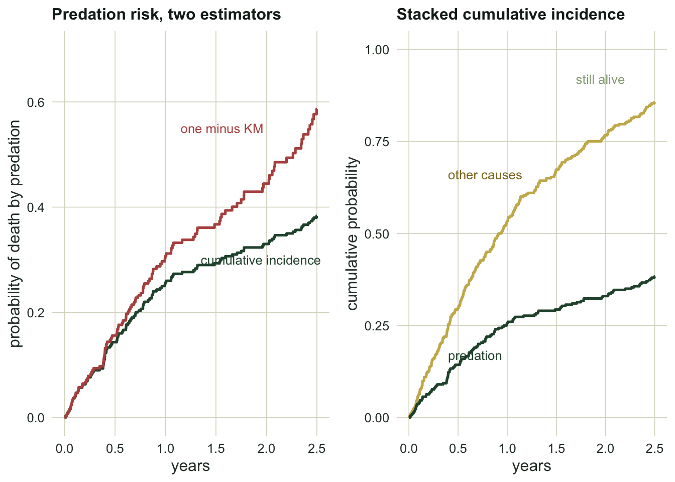
The naive curve puts the probability of death by predation at 0.586. The cumulative incidence function puts it at 0.383. That is an overstatement of 53 percent, and it is not a fluke of this sample; the mechanism is structural.

One minus Kaplan-Meier asks “what fraction would eventually be predated if other-cause deaths were merely a temporary interruption?” But an animal killed by disease is not interrupted; it is gone, and can never be predated. Censoring those animals treats them as if they re-enter the predation risk set later, which inflates the estimate. The CIF keeps the accounting honest: the other-cause deaths stay out of the numerator, and the two causes plus the survivors add up exactly to one.

cif_total  <- aj_cif_pred + aj_cif_other
surv_total <- 1 - exp(-(rate_pred + rate_other) * tau)

Here the two cumulative incidences sum to 0.857, which matches one minus the overall survival, 0.847. The naive curve has no such guarantee: add up one minus Kaplan-Meier across both causes and the total can exceed one.

Figure 1: Left: one minus Kaplan-Meier for predation overstates the risk relative to the cumulative incidence function. Right: the stacked cumulative incidence splits total mortality into the two causes, always summing to one minus overall survival.

Two hazards, two questions

The modelling side hides a subtler point. Add a covariate, say a habitat indicator that raises the risk of both causes, and ask how it affects predation. There are two hazards you could model, and they do not agree.

The cause-specific hazard is the instantaneous predation rate among animals still alive and at risk; you fit it with a Cox model that censors the other-cause deaths. The subdistribution hazard of Fine and Gray is built so that its coefficient maps directly onto the cumulative incidence; it keeps animals who died of a competing cause in the risk set, with a weight that decays over time.

set.seed(42562)
nb <- 1200
x <- rbinom(nb, 1, 0.5)
h_pred  <- 0.25 * exp(log(1.8) * x)
h_other <- 0.40 * exp(log(1.8) * x)
taub <- 3
tp <- rexp(nb, h_pred); to <- rexp(nb, h_other)
tb <- pmin(tp, to, taub)
cb <- ifelse(tb == taub, 0L, ifelse(tp < to, 1L, 2L))
db <- data.frame(time = tb, cause = cb, x = x)

csh <- coxph(Surv(time, cause == 1) ~ x, data = db)
csh_hr <- exp(coef(csh)); csh_ci <- exp(confint(csh))

evb <- factor(cb, levels = c(0, 1, 2), labels = c("censor", "pred", "other"))
fg <- finegray(Surv(time, evb) ~ ., data = data.frame(time = tb, x = x, evb = evb),
               etype = "pred")
fgm <- coxph(Surv(fgstart, fgstop, fgstatus) ~ x, weight = fgwt, data = fg)
fg_hr <- exp(coef(fgm)); fg_ci <- exp(confint(fgm))

cif_group <- function(sub) {
  e <- factor(sub$cause, levels = c(0, 1, 2), labels = c("c", "pred", "other"))
  a <- survfit(Surv(sub$time, e) ~ 1)
  s <- summary(a, times = taub, extend = TRUE)
  s$pstate[, which(a$states == "pred")]
}
cif_x0 <- cif_group(db[db$x == 0, ])
cif_x1 <- cif_group(db[db$x == 1, ])

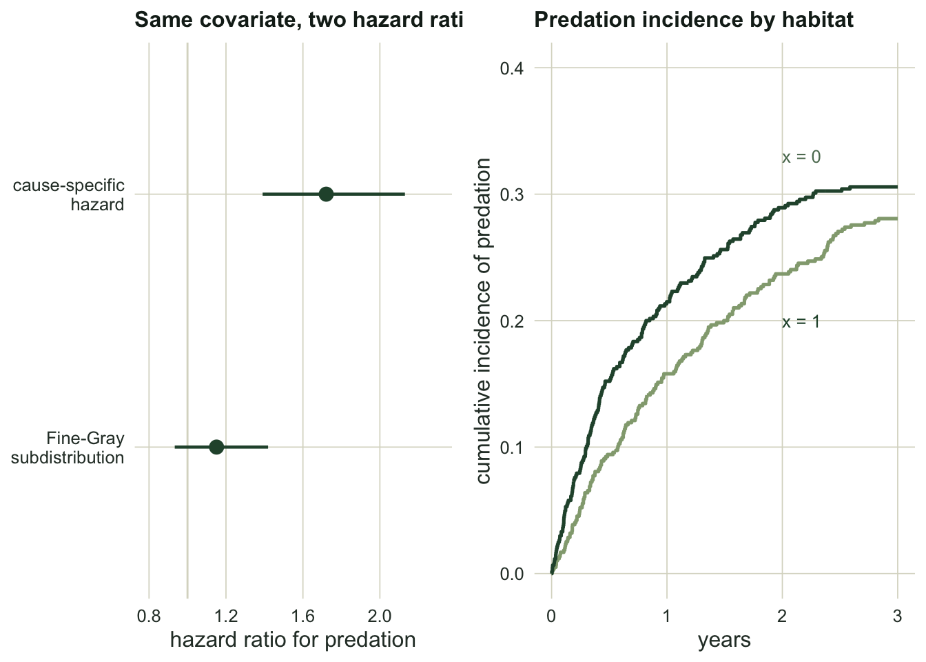
The habitat covariate raises the cause-specific predation hazard by a clear margin: the cause-specific hazard ratio is 1.72 (95 percent interval 1.39 to 2.13). Read as a rate among survivors, animals in this habitat are predated faster.

Yet the Fine-Gray subdistribution hazard ratio is only 1.15 (interval 0.93 to 1.42, spanning one), and the cumulative incidence of predation barely moves: 0.281 at x equal to zero against 0.306 at x equal to one. The reason is the competing cause. The same habitat also raises other-cause mortality, so animals there tend to die of something else before a predator reaches them. The elevated predation rate is cancelled by faster removal through the competing risk, and the probability of actually dying by predation stays flat.

Figure 2: Left: the cause-specific hazard ratio for the covariate sits clearly above one, while the Fine-Gray subdistribution ratio is close to one. Right: the cumulative incidence of predation is nearly identical across the covariate, because the covariate also raises the competing cause.

How reliable is the overstatement

To confirm that one minus Kaplan-Meier is systematically biased rather than merely unlucky here, repeat the first scenario a thousand times and compare both estimators against the known cumulative incidence.

set.seed(425699)
B <- 1000
truth <- (rate_pred / (rate_pred + rate_other)) *
  (1 - exp(-(rate_pred + rate_other) * tau))
naive_mc <- aj_mc <- numeric(B)
for (b in 1:B) {
  tp <- rexp(300, rate_pred); to <- rexp(300, rate_other)
  tm <- pmin(tp, to, tau)
  cc <- ifelse(tm == tau, 0L, ifelse(tp < to, 1L, 2L))
  naive_mc[b] <- 1 - summary(survfit(Surv(tm, cc == 1) ~ 1), times = tau, extend = TRUE)$surv
  e <- factor(cc, levels = c(0, 1, 2), labels = c("c", "p", "o"))
  aa <- survfit(Surv(tm, e) ~ 1)
  aj_mc[b] <- summary(aa, times = tau, extend = TRUE)$pstate[, which(aa$states == "p")]
}
naive_bias <- mean(naive_mc) - truth
aj_bias <- mean(aj_mc) - truth

Against a true cumulative incidence of 0.339, one minus Kaplan-Meier averages 0.528, a bias of +0.190. The Aalen-Johansen cumulative incidence averages 0.339, a bias of +0.000. The overstatement is a property of the estimator, not the draw.

What to take away

With competing causes of death the right target is the cumulative incidence function, estimated by Aalen-Johansen, not one minus Kaplan-Meier. When you model a covariate, keep the two hazards distinct: the cause-specific hazard describes the rate among survivors and answers a mechanistic question (“does this habitat make predation faster?”), while the Fine-Gray subdistribution hazard tracks the cumulative incidence and answers a population question (“are more animals in this habitat actually killed by predators?”). They can disagree, and each is right about its own question. Report the cumulative incidence when the quantity of interest is how many animals a cause removes, and never read one minus Kaplan-Meier as if a competing death were a temporary pause.

References

Aalen, O. O. and Johansen, S. (1978) An empirical transition matrix for non-homogeneous Markov chains based on censored observations. Scandinavian Journal of Statistics 5, 141-150.

Andersen, P. K., Geskus, R. B., de Witte, T. and Putter, H. (2012) Competing risks in epidemiology: possibilities and pitfalls. International Journal of Epidemiology 41, 861-870. https://doi.org/10.1093/ije/dyr213

Austin, P. C., Lee, D. S. and Fine, J. P. (2016) Introduction to the analysis of survival data in the presence of competing risks. Circulation 133, 601-609. https://doi.org/10.1161/CIRCULATIONAHA.115.017719

Fine, J. P. and Gray, R. J. (1999) A proportional hazards model for the subdistribution of a competing risk. Journal of the American Statistical Association 94, 496-509. https://doi.org/10.1080/01621459.1999.10474144

Gray, R. J. (1988) A class of K-sample tests for comparing the cumulative incidence of a competing risk. Annals of Statistics 16, 1141-1154. https://doi.org/10.1214/aos/1176350951

Heisey, D. M. and Patterson, B. R. (2006) A review of methods to estimate cause-specific mortality in presence of competing risks. Journal of Wildlife Management 70, 1544-1555.

Putter, H., Fiocco, M. and Geskus, R. B. (2007) Tutorial in biostatistics: competing risks and multi-state models. Statistics in Medicine 26, 2389-2430. https://doi.org/10.1002/sim.2712

Related tutorials

• Parametric survival and the AFT model
• Frailty and recurrent event models
• Checking a survival model
• Cox proportional hazards and the PH assumption

## References

Aalen OO, Johansen S 1978 Scandinavian Journal of Statistics 5:141-150
Andersen PK, Geskus RB, de Witte T, Putter H 2012 International Journal of Epidemiology 41:861-870 (10.1093/ije/dyr213)
Austin PC, Lee DS, Fine JP 2016 Circulation 133:601-609 (10.1161/CIRCULATIONAHA.115.017719)
Fine JP, Gray RJ 1999 Journal of the American Statistical Association 94:496-509 (10.1080/01621459.1999.10474144)
Gray RJ 1988 Annals of Statistics 16:1141-1154 (10.1214/aos/1176350951)
Heisey DM, Patterson BR 2006 Journal of Wildlife Management 70:1544-1555 (10.2193/0022-541X(2006)70[1544:AROMTE]2.0.CO;2)
Putter H, Fiocco M, Geskus RB 2007 Statistics in Medicine 26:2389-2430 (10.1002/sim.2712)