library(ggplot2)
library(patchwork)
library(survival)

te_paper  <- "#f5f4ee"
te_ink    <- "#16241d"
te_body   <- "#2c3a31"
te_forest <- "#275139"
te_rust   <- "#b5534e"
te_gold   <- "#c9b458"
te_line   <- "#dad9ca"

theme_datasheet <- function() {
  theme_minimal(base_size = 12) +
    theme(plot.background  = element_rect(fill = te_paper, colour = NA),
          panel.background = element_rect(fill = te_paper, colour = NA),
          panel.grid.major = element_line(colour = te_line, linewidth = 0.3),
          panel.grid.minor = element_blank(),
          text             = element_text(colour = te_body),
          plot.title       = element_text(colour = te_ink, face = "bold"),
          plot.subtitle    = element_text(colour = te_body),
          axis.text        = element_text(colour = te_body))
}Interval-censored survival from visit data
R
survival analysis
censoring
survival
simulation
ecology tutorial
Coding a death found on a tracking visit at the interval midpoint can flip a falling hazard into a rising one. Fitting interval-censored Weibull survival in R.
A batch of two hundred captive-reared partridges is released on a farm estate, each bird carrying a radio tag. A field worker walks the tracking route every six days and records, for each bird, whether the signal still comes from a living bird or from a carcass. After thirty-six days the tags are collected. The data sheet holds, for every dead bird, the last visit it was seen alive and the visit that found it dead. The death itself happened somewhere in between, and nobody saw when.
The question the release team wants answered is the shape of the risk. If most birds die in the first days after release and the survivors then settle, the hazard falls with time, and the management answer is a softer release: a pen, supplementary food, a longer acclimatisation. If the risk rises instead, the birds are running out of something, and the answer is different. A Weibull model reports exactly this in one parameter, its shape: below one the hazard falls, above one it rises. So the spreadsheet gets a death time column, filled with the midpoint between the two visits or, more often, with the date of the visit that found the carcass, and the column goes into survreg.
This post measures what those two codings do to the Weibull shape and to the median survival time, and compares them with the likelihood that uses the interval as an interval. The site has already met the underlying idea. Rounded and coarsened measurements writes the interval-censored likelihood for normal data read off a fixed grid, and finds that the grid leaves the mean alone and damages the shape of the distribution. Here the grid is the visit schedule, it is coarse relative to the event times, and the damage is to the direction of the hazard, the one thing a Weibull shape parameter is fitted to report. The post on time-varying covariates in survival states the problem and steps around it: when a state change is known only to lie between visits, it says, that is interval censoring, a different problem it does not solve. The Weibull model itself, its two readings and its right-censored likelihood are set out in parametric survival and the AFT model; that post assumes every death time is known exactly. And census interval bias in tree mortality rates is about a rate computed from counts at two censuses, where the interval length interacts with unmeasured frailty; nothing there is a death time.
A release tracked every six days
The generating model is a Weibull with scale 10 days and shape 0.8, so the hazard falls over time and the true median survival is fixed by the two parameters. The study runs for 36 days. Visits come every w days. Two schedules are simulated because they are the two ways a release meets a tracking rota. In the aligned schedule the release day is itself a visit, so the first check falls w days later. In the offset schedule the rota runs on its own calendar and the first check after release comes after a uniform delay between zero and w days. All of these constants were fixed before any simulation was run.
lambda_true <- 10      # Weibull scale, days
shape_dec   <- 0.8     # falling hazard
shape_inc   <- 2.5     # rising hazard, used later
n_bird      <- 200
t_end       <- 36      # days of tracking
w_main      <- 6       # days between visits in the worked example

median_weib <- function(shape, scl) scl * log(2)^(1 / shape)
surv_weib   <- function(x, shape, scl) exp(-(x / scl)^shape)
haz_weib    <- function(x, shape, scl) (shape / scl) * (x / scl)^(shape - 1)

# left = last visit seen alive (NA if dead before the first check),
# right = visit that found the bird dead (NA if alive at the last check)
code_visits <- function(t_death, w, first_check) {
  last_check <- first_check + floor((t_end - first_check) / w) * w
  alive <- t_death > last_check
  right <- pmax(ceiling((t_death - first_check) / w) * w + first_check, first_check)
  left  <- right - w
  left[t_death <= first_check] <- NA
  right[alive] <- NA
  left[alive]  <- last_check
  data.frame(t_death, left, right, alive, before_first = is.na(left),
             last_check, first_check)
}
A bird alive at the last check is right-censored there: its left end is the last check and its right end is missing. A bird dead before the first check has no visit at which it was seen alive after release, so its left end is missing too. That second case is the gotcha of Surv(type = "interval2"): writing a zero instead of NA for the left end makes survreg refuse the Weibull fit, because a Weibull time cannot be zero (the next worked example tries it), and writing a small positive number quietly changes the data.
Five fits are made to every dataset. The exact fit sees the true death times, censored at the last check, and is the reference no field study has. The midpoint coding puts each death halfway between the two visits, counting release as time zero for birds that died before the first check. The detection coding puts each death on the visit that found it. A fourth, hybrid coding is there to answer a question the results raise: it treats deaths before the first check as left-censored and uses midpoints everywhere else. The fifth is the interval-censored likelihood.
shape_of <- function(f) 1 / f$scale
lam_of   <- function(f) exp(unname(coef(f)[1]))

fit_codings <- function(d) {
  ev    <- !d$alive
  lo    <- ifelse(d$before_first, 0, d$left)
  t_mid <- ifelse(ev, (lo + d$right) / 2, d$last_check)
  t_det <- ifelse(ev, d$right, d$last_check)
  hyb_l <- ifelse(d$before_first, NA, ifelse(ev, t_mid, d$last_check))
  hyb_r <- ifelse(d$before_first, d$first_check, ifelse(ev, t_mid, NA))
  n_warn <- 0
  quiet_fit <- function(fml) withCallingHandlers(
    survreg(fml, dist = "weibull"),
    warning = function(wm) { n_warn <<- n_warn + 1; invokeRestart("muffleWarning") })
  fits <- list(
    exact     = quiet_fit(Surv(pmin(d$t_death, d$last_check), ev) ~ 1),
    midpoint  = quiet_fit(Surv(t_mid, ev) ~ 1),
    detection = quiet_fit(Surv(t_det, ev) ~ 1),
    hybrid    = quiet_fit(Surv(hyb_l, hyb_r, type = "interval2") ~ 1),
    interval2 = quiet_fit(Surv(d$left, d$right, type = "interval2") ~ 1))
  f_ic  <- fits$interval2
  log_s <- log(f_ic$scale)
  se_ls <- sqrt(vcov(f_ic)["Log(scale)", "Log(scale)"])
  list(shape = vapply(fits, shape_of, 0), lam = vapply(fits, lam_of, 0),
       ci_shape = sort(1 / exp(log_s + c(-1, 1) * qnorm(0.975) * se_ls)), se_ls = se_ls,
       n_warn = n_warn, fits = fits)
}
survreg parameterises the Weibull as a log-linear model: the log time has a location equal to the intercept and an extreme value error multiplied by what it calls the scale. The Weibull shape is the reciprocal of that scale and the Weibull scale in days is the exponential of the intercept, which is the conversion in shape_of and lam_of. The next chunk checks the conversion rather than trusting it.
set.seed(20260825)
one_d   <- code_visits(lambda_true * rexp(n_bird)^(1 / shape_dec), w_main, w_main)
one_fit <- fit_codings(one_d)

n_before <- sum(one_d$before_first)
n_alive  <- sum(one_d$alive)
n_inner  <- n_bird - n_before - n_alive
med_true <- median_weib(shape_dec, lambda_true)
one_med  <- median_weib(one_fit$shape, one_fit$lam)

# the conversion: simulate from the fitted exact model and refit
set.seed(99)
chk_t   <- one_fit$lam[["exact"]] * rexp(200000)^(1 / one_fit$shape[["exact"]])
chk_fit <- survreg(Surv(chk_t) ~ 1, dist = "weibull")
zero_try <- tryCatch(
  survreg(Surv(ifelse(one_d$before_first, 0, one_d$left), one_d$right,
               type = "interval2") ~ 1, dist = "weibull"),
  error = function(e) conditionMessage(e))
zero_msg <- if (is.character(zero_try)) {
  paste0('`survreg` stops with the message "', zero_try, '"')
} else {
  "this version of `survival` accepts it without an error, so nothing in the output warns that the coding is wrong"
}
chk_gap <- max(abs(c(shape_of(chk_fit) / one_fit$shape[["exact"]],
                     lam_of(chk_fit) / one_fit$lam[["exact"]]) - 1))
In this release 95 of the 200 birds died before the first check, 90 died between two later checks and 15 were alive at the end. The true shape is 0.8 and the true median survival is 6.32 days. The exact fit returns a shape of 0.796, and the interval-censored fit 0.780. The midpoint coding returns 1.029 and the detection coding 1.395: both above one, both describing a hazard that rises. Their medians are 8.40 and 12.24 days, against 6.48 from the interval-censored fit.
As a check on the conversion, a sample of 200000 times drawn from the exact fit’s shape and scale, refitted by survreg, returns both parameters to within a relative error of 0.0017. The same chunk also codes the birds dead before the first check with a left end of zero, and this version of survival accepts it without an error, so nothing in the output warns that the coding is wrong.
t_grid <- seq(0.5, t_end, length.out = 300)
haz_labs <- c(truth = "truth", exact = "exact death times",
              midpoint = "midpoint coding", detection = "detection visit coding",
              interval2 = "interval-censored")
haz_df <- do.call(rbind, lapply(names(haz_labs), function(k) {
  if (k == "truth") h <- haz_weib(t_grid, shape_dec, lambda_true)
  else h <- haz_weib(t_grid, one_fit$shape[[k]], one_fit$lam[[k]])
  data.frame(t = t_grid, hazard = h, coding = haz_labs[[k]])
}))
haz_df$coding <- factor(haz_df$coding, levels = unname(haz_labs))

ggplot(haz_df, aes(t, hazard, colour = coding, linetype = coding)) +
  geom_vline(xintercept = seq(w_main, t_end, by = w_main), colour = te_line,
             linewidth = 0.6) +
  geom_line(linewidth = 0.9) +
  scale_colour_manual(values = c(te_ink, "grey55", te_gold, te_rust, te_forest),
                      name = NULL) +
  scale_linetype_manual(values = c("dashed", "solid", "solid", "solid", "solid"),
                        name = NULL) +
  scale_y_log10() +
  labs(x = "days since release", y = "hazard per day (log scale)",
       title = "Two codings turn a falling hazard into a rising one",
       subtitle = "pale vertical lines: tracking visits") +
  theme_datasheet() +
  theme(legend.position = "bottom") +
  guides(colour = guide_legend(nrow = 2))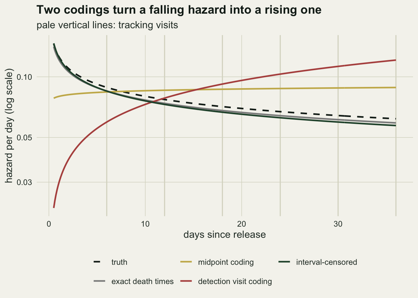
The likelihood in three lines
A bird last seen alive at the left end and found dead at the right end contributes the probability of dying in that interval, the survival function at the left end minus the survival function at the right end. A bird dead before the first check has a left survival of one; a bird alive at the end has a right survival of zero. Lindsey and Ryan (1998) set out this likelihood and the ways around it. Written by hand, and maximised with optim, it should give what survreg gives.
nll_ic <- function(par, d) {
  s_left  <- ifelse(is.na(d$left), 1, surv_weib(d$left, exp(par[1]), exp(par[2])))
  s_right <- ifelse(is.na(d$right), 0, surv_weib(d$right, exp(par[1]), exp(par[2])))
  -sum(log(s_left - s_right))
}
hand_opt <- optim(c(0, log(median(one_d$right, na.rm = TRUE))), nll_ic, d = one_d,
                  method = "BFGS")
ll_survreg <- one_fit$fits$interval2$loglik[2]
ll_hand_at <- -nll_ic(log(c(one_fit$shape[["interval2"]], one_fit$lam[["interval2"]])),
                      one_d)
hand_shape <- exp(hand_opt$par[1])
hand_lam   <- exp(hand_opt$par[2])
At survreg’s estimates, the hand-written log-likelihood is -304.631723 and survreg reports -304.631723. Maximising the hand version independently gives a shape of 0.7803 and a scale of 10.3575 days, against 0.7803 and 10.3575 from survreg. So type = "interval2" is this likelihood and nothing more, and the shape conversion above is the right one.
Over replicates the midpoint reverses the hazard
One release proves nothing about a coding. The next chunk repeats the whole release 400 times for each combination of true shape, visit interval and schedule. Each replicate gets its own death times, and in the offset schedule its own first-check delay. Estimates are summarised by their median over replicates, because at the coarsest schedules some fits wander far.
widths <- c(3, 6, 9, 12)
n_rep  <- 400
codings <- c("exact", "midpoint", "detection", "hybrid", "interval2")

run_cell <- function(shape_true, w, schedule) {
  rows <- lapply(seq_len(n_rep), function(i) {
    fc <- if (schedule == "aligned") w else runif(1, 0, w)
    d  <- code_visits(lambda_true * rexp(n_bird)^(1 / shape_true), w, fc)
    f  <- fit_codings(d)
    c(setNames(f$shape, paste0("shape_", codings)),
      setNames(median_weib(f$shape, f$lam), paste0("med_", codings)),
      cover = f$ci_shape[1] < shape_true & shape_true < f$ci_shape[2],
      ci_lo = f$ci_shape[1], ci_hi = f$ci_shape[2], se_ls = f$se_ls,
      warn = f$n_warn, p_before = mean(d$before_first),
      # birds not yet found dead at the second check (alive at the end included)
      n_late = sum(is.na(d$right) | d$right > d$first_check + w))
  })
  data.frame(shape_true, w, schedule, do.call(rbind, rows))
}

cells <- expand.grid(shape_true = c(shape_dec, shape_inc), w = widths,
                     schedule = c("aligned", "offset"), stringsAsFactors = FALSE)
set.seed(4471)
sim_all <- do.call(rbind, Map(run_cell, cells$shape_true, cells$w, cells$schedule))
n_warn_total <- sum(sim_all$warn)
cell_key <- paste(sim_all$shape_true, sim_all$w, sim_all$schedule)
summ <- do.call(rbind, lapply(split(sim_all, cell_key), function(s) {
out <- data.frame(shape_true = s$shape_true[1], w = s$w[1], schedule = s$schedule[1],
coding = codings)
sh <- as.matrix(s[, paste0("shape_", codings)])
md <- as.matrix(s[, paste0("med_", codings)])
out$shape_med <- apply(sh, 2, median)
out$shape_q1 <- apply(sh, 2, quantile, 0.25)
out$shape_q3 <- apply(sh, 2, quantile, 0.75)
out$p_rev <- colMeans(sh > 1)
out$med_bias <- 100 * (apply(md, 2, median, na.rm = TRUE) /
median_weib(s$shape_true[1], lambda_true) - 1)
out$cover <- mean(s$cover)
out$p_before <- mean(s$p_before)
out
}))
rownames(summ) <- NULL
pick <- function(col, shp, w, sch, cod) {
summ[[col]][summ$shape_true == shp & summ$w == w & summ$schedule == sch &
summ$coding == cod]
}
mc_se <- function(p) sqrt(p * (1 - p) / n_rep)cod_lab <- c(exact = "exact death times", midpoint = "midpoint coding",
detection = "detection visit coding", interval2 = "interval-censored")
cod_col <- c("grey55", te_gold, te_rust, te_forest)
sw <- summ[summ$shape_true == shape_dec & summ$coding %in% names(cod_lab), ]
sw$coding <- factor(cod_lab[sw$coding], levels = unname(cod_lab))
sw$schedule <- factor(ifelse(sw$schedule == "aligned", "release on a visit day",
"release between visits"),
levels = c("release on a visit day", "release between visits"))
ggplot(sw, aes(w, shape_med, colour = coding)) +
geom_hline(yintercept = 1, colour = te_ink, linewidth = 0.5) +
geom_hline(yintercept = shape_dec, colour = te_ink, linetype = "dashed",
linewidth = 0.5) +
geom_errorbar(aes(ymin = shape_q1, ymax = shape_q3), width = 0.8,
position = position_dodge(width = 1.6), linewidth = 0.6) +
geom_point(size = 2.2, position = position_dodge(width = 1.6)) +
geom_line(position = position_dodge(width = 1.6), linewidth = 0.6) +
facet_wrap(~ schedule) +
scale_colour_manual(values = cod_col, name = NULL) +
scale_x_continuous(breaks = widths) +
labs(x = "days between tracking visits", y = "estimated Weibull shape",
title = "The midpoint crosses one as visits spread out",
subtitle = "solid line: shape 1, constant hazard; dashed line: true shape 0.8") +
theme_datasheet() +
theme(legend.position = "bottom") +
guides(colour = guide_legend(nrow = 2))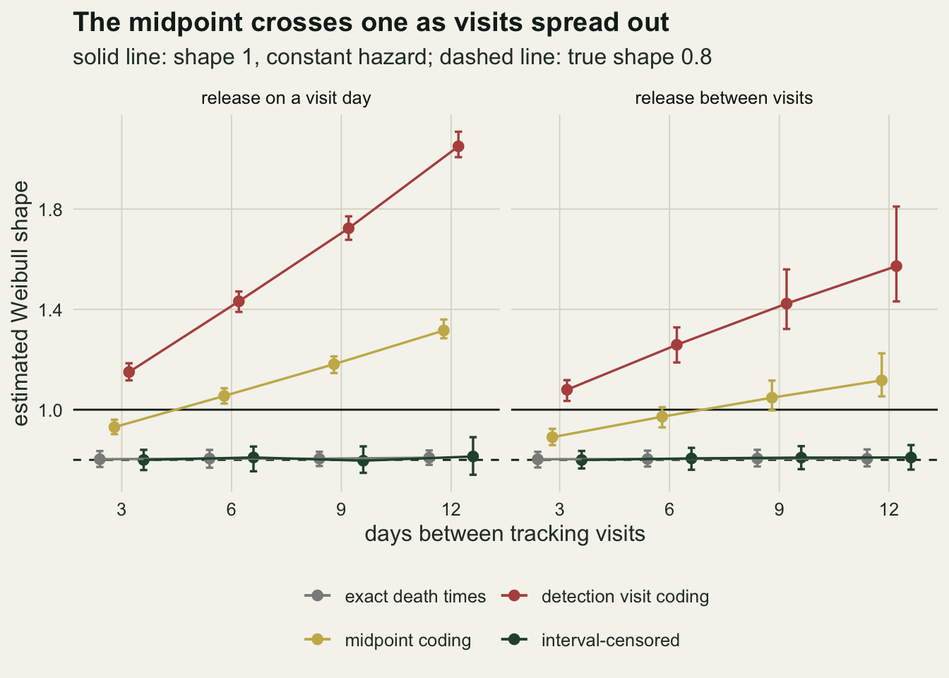
cells_dec <- summ$shape_true == shape_dec & summ$coding == "interval2"
ic_dec_lo <- min(summ$shape_med[cells_dec])
ic_dec_hi <- max(summ$shape_med[cells_dec])
p_mid6 <- pick("p_rev", shape_dec, 6, "aligned", "midpoint")
p_mid6_off <- pick("p_rev", shape_dec, 6, "offset", "midpoint")
p_mid9_off <- pick("p_rev", shape_dec, 9, "offset", "midpoint")
p_mid12_off <- pick("p_rev", shape_dec, 12, "offset", "midpoint")
Over 400 releases in each cell, the median interval-censored shape stays between 0.797 and 0.814 across all eight combinations of visit interval and schedule, against a true 0.8. The two codings do not. With a release on a visit day and checks every 3 days, the midpoint coding already pulls the median shape up to 0.931. At 6 days it is 1.055, and the fitted shape exceeds one in 0.882 of the releases (Monte Carlo standard error 0.016): the analysis reports a rising hazard for a population whose hazard falls. At 9 and 12 days every one of the 400 releases does. The detection coding is above one at every interval, with a median shape of 1.150 at three days and 2.050 at twelve.
The median survival time tells the same story in days. At six-day visits on the aligned schedule the midpoint coding overstates it by 29.6 per cent and the detection coding by 90.1 per cent, while the interval-censored fit is off by 0.8 per cent.
Releasing between visits softens the midpoint coding without rescuing it. At six days the fitted shape exceeds one in 0.305 of the offset releases, at nine days in 0.740 and at twelve in 0.912. So the reversal is not a quirk of releasing on a visit day, but the schedule changes how soon it arrives, and that points at where it comes from.
The first interval does the damage
On the aligned schedule the first check falls a full interval after release, and with a falling hazard that interval holds a large share of all deaths: 0.49 of the birds on average at six-day visits, 0.68 at twelve. Inside that interval the deaths are packed towards release day, because that is where the hazard is highest. The midpoint coding moves all of them to the middle of the interval. The shortest survival times, which are the evidence that the hazard falls, disappear from the data, and the Weibull fit has to explain a population in which almost nobody dies in the first days and many die just after. A rising hazard explains that.
The hybrid coding tests this directly. It keeps the midpoint for every interval except the one before the first check, where it uses the left-censored interval instead. On the aligned schedule at six days its median shape is 0.819, with a fitted shape above one in 0.0025 of releases, and at twelve days 0.813 and 0.035. For this schedule, almost the whole reversal comes from one interval.
On the offset schedule the hybrid coding is not clean. Its median shape is 0.844 at six days and 0.871 at twelve, where the shape exceeds one in 0.155 of releases. When the first check comes a day or two after release, the second interval also begins where the hazard is still falling fast, and its midpoint carries a smaller copy of the same error. A likely reading, not tested here because no coding repairs the second interval alone, is that midpoint coding does its harm in the intervals where the density of death times changes steeply across the interval, which for a falling hazard means the intervals nearest release. Repairing the first one is a diagnostic, not a method: the interval-censored likelihood repairs all of them at once, and on both schedules its reversal rate never exceeds 0.037, the value at twelve-day visits where the estimates are simply less precise.
rev_lab <- c(midpoint = "midpoint coding", detection = "detection visit coding",
             hybrid = "midpoint, first interval left-censored",
             interval2 = "interval-censored")
rv <- summ[summ$shape_true == shape_dec & summ$coding %in% names(rev_lab), ]
rv$coding <- factor(rev_lab[rv$coding], levels = unname(rev_lab))
rv$schedule <- factor(ifelse(rv$schedule == "aligned", "release on a visit day",
                             "release between visits"),
                      levels = c("release on a visit day", "release between visits"))
rv$se <- mc_se(rv$p_rev)

ggplot(rv, aes(w, p_rev, colour = coding)) +
  geom_line(linewidth = 0.7) +
  geom_errorbar(aes(ymin = pmax(p_rev - 2 * se, 0), ymax = pmin(p_rev + 2 * se, 1)),
                width = 0.5, linewidth = 0.5) +
  geom_point(size = 2.2) +
  facet_wrap(~ schedule) +
  scale_colour_manual(values = c(te_gold, te_rust, te_ink, te_forest), name = NULL) +
  scale_x_continuous(breaks = widths) +
  labs(x = "days between tracking visits",
       y = "share of releases with fitted shape above 1",
       title = "Most midpoint reversals come from the first interval") +
  theme_datasheet() +
  theme(legend.position = "bottom") +
  guides(colour = guide_legend(nrow = 2))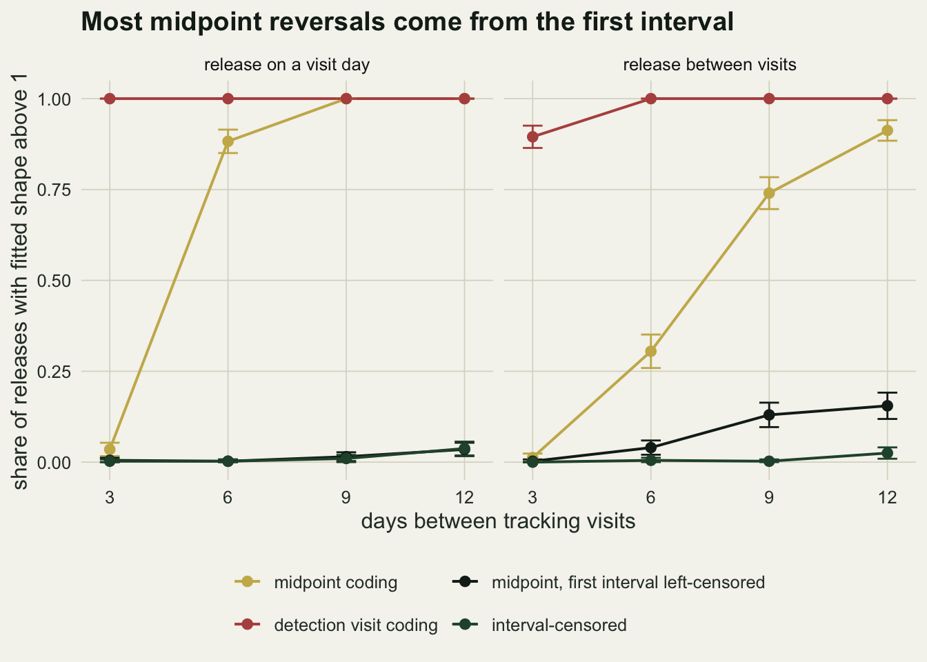
A rising hazard loses its shape and keeps its median
shape_err <- function(w, sch, cod) 100 * (pick("shape_med", shape_inc, w, sch, cod) / shape_inc - 1)
dead_by_24 <- 1 - surv_weib(24, shape_inc, lambda_true)
rise_min_share <- min(summ$p_rev[summ$shape_true == shape_inc])

# the aligned twelve-day cell with a rising hazard
fail_cell <- sim_all[sim_all$shape_true == shape_inc & sim_all$w == 12 &
                     sim_all$schedule == "aligned", ]
no_late   <- fail_cell$n_late == 0
p_no_late <- mean(no_late)
n_late_rel <- sum(!no_late)
stop_range <- range(fail_cell$shape_interval2[no_late])
stop_med   <- median(fail_cell$shape_interval2[no_late])
late_med   <- median(fail_cell$shape_interval2[!no_late])
warn_no_late <- sum(fail_cell$warn[no_late] > 0)
off12_q3 <- pick("shape_q3", shape_inc, 12, "offset", "interval2")
off_cell <- sim_all[sim_all$shape_true == shape_inc & sim_all$w == 12 &
                    sim_all$schedule == "offset", ]
p_no_late_off <- mean(off_cell$n_late == 0)
off_est_med   <- median(off_cell$shape_interval2[off_cell$n_late > 0])
p_no_late9 <- mean(sim_all$n_late[sim_all$shape_true == shape_inc & sim_all$w == 9 &
                                   sim_all$schedule == "aligned"] == 0)
The second case is a population whose hazard rises, such as adult butterflies marked on a transect and resighted on visits, simulated with the same scale and a shape of 2.5. Fewer animals die before the first check, 0.24 of them at six-day visits on the aligned schedule against 0.49 with the falling hazard, and a midpoint cannot turn a rising hazard into a falling one in these runs: across all 40 combinations of interval, schedule and coding, the smallest share of fitted shapes above one is 1.000.
The damage is selective instead. At six-day visits the midpoint coding lowers the median shape by 9.2 per cent and at nine days by 19.2 per cent, while its median survival time is too short by only 1.7 and 3.6 per cent. A reader who wants the median gets a usable number; a reader who wants to know how fast the risk accelerates with age does not. The detection coding biases both: at six days the shape is 24.6 per cent too high and the median survival 36.4 per cent too long. The interval-censored fit is within 1.4 per cent on the shape at three, six and nine days.
At twelve days on the aligned schedule there is no estimate to report. The visits fall on days 12, 24 and 36, and under the true model a fraction 0.9999 of the animals is dead by day 24. In 0.968 of the 400 releases not one bird is still unaccounted for at the second check: every animal is either found dead at day 12 or found dead at day 24. The interval likelihood then has no maximum. It keeps rising as the shape grows, because a steeper curve can hold the share dead by day 12 at its observed value while pushing survival at day 24 ever closer to zero, and survreg stops where its steps become small. In those releases the reported shape runs from 4.15 to 5.69 (median 4.58); that is where the optimiser stopped, not an estimate, and only 0 of these 387 releases produced a warning from any of the five fits. In the 13 releases with at least one bird past day 24, the median shape is 1.72, below the truth. The likelihood is not wrong; this visit schedule cannot identify a shape. The nine-day aligned schedule, with its second check on day 18, is not safe either: nobody is past that check in 0.095 of its releases, and there too the reported shape is a stopping point. On the offset schedule the first check comes sooner after release, so the second check falls before day 24 and more birds outlast it. The same boundary still applies in the 0.295 of offset releases with nobody past the second check, where the reported shapes are stopping points again, and a quarter of all offset fits exceed a shape of 3.99. In the offset releases with at least one bird past the second check the median shape is 2.49; the median of 2.64 over all of them mixes estimates with stopping points.
ri <- summ[summ$shape_true == shape_inc & summ$schedule == "aligned" &
           summ$coding %in% c("midpoint", "detection", "interval2"), ]
ri$coding <- factor(cod_lab[ri$coding], levels = unname(cod_lab[-1]))
ri$shape_bias <- 100 * (ri$shape_med / shape_inc - 1)
ri <- ri[!(ri$coding == "interval-censored" & ri$w == 12), ]  # not estimable

p_shape <- ggplot(ri, aes(w, shape_bias, colour = coding)) +
  geom_hline(yintercept = 0, colour = te_ink, linewidth = 0.5) +
  geom_line(linewidth = 0.7) + geom_point(size = 2.2) +
  scale_colour_manual(values = cod_col[-1], name = NULL) +
  scale_x_continuous(breaks = widths) +
  labs(x = "days between tracking visits", y = "per cent error, median shape",
       title = "Shape") +
  theme_datasheet()
p_med <- ggplot(ri, aes(w, med_bias, colour = coding)) +
  geom_hline(yintercept = 0, colour = te_ink, linewidth = 0.5) +
  geom_line(linewidth = 0.7) + geom_point(size = 2.2) +
  scale_colour_manual(values = cod_col[-1], name = NULL) +
  scale_x_continuous(breaks = widths) +
  labs(x = "days between tracking visits", y = "per cent error, median survival",
       title = "Median survival") +
  theme_datasheet()
(p_shape | p_med) + plot_layout(guides = "collect") +
  plot_annotation(theme = theme_datasheet()) &
  theme(legend.position = "bottom")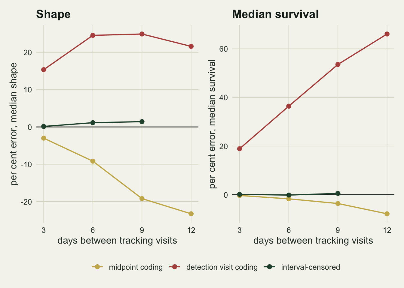
Is the interval-censored interval honest?
cov_cells <- summ[summ$coding == "interval2", ]
cov_bad   <- cov_cells$shape_true == shape_inc & cov_cells$w == 12 &
             cov_cells$schedule == "aligned"
cov_lo <- min(cov_cells$cover[!cov_bad])
cov_hi <- max(cov_cells$cover[!cov_bad])
cov_se <- mc_se(0.95)
cov_within <- sum(abs(cov_cells$cover[!cov_bad] - 0.95) <= 2 * cov_se)
cov_top <- cov_cells[!cov_bad, ][which.max(cov_cells$cover[!cov_bad]), ]
warn_by_sch <- tapply(sim_all$warn[sim_all$shape_true == shape_inc & sim_all$w == 12],
                      sim_all$schedule[sim_all$shape_true == shape_inc & sim_all$w == 12], sum)
p_se_zero <- mean(fail_cell$se_ls[no_late] < 1e-6)
p_hi_inf  <- mean(is.infinite(fail_cell$ci_hi[no_late]))
survreg gives a standard error for the log of its scale. The interval for the shape used here is the Wald interval on that log scale, 95 per cent, turned into an interval for the shape by the reciprocal of its exponential; its ends swap order under that transformation, which is why the code sorts them. Across the fifteen cells other than the failed one, the interval covers the true shape in between 0.925 and 0.980 of releases. The Monte Carlo standard error of a coverage near 0.95 with 400 releases is 0.011, and 13 of the fifteen values lie within two standard errors of the nominal level. The exception is the highest, in the cell with a rising hazard and 9-day visits on the aligned schedule, and it errs on the conservative side. In the failed cell the Wald interval is degenerate. Among the releases with nobody past the second check, its standard error is numerically zero in 0.553 of them, so the interval collapses onto the stopping value, and its upper end is infinite in 0.354. The coverage of 0.435 in that cell is mostly a mixture of those two cases and means nothing.
survreg issued 34 warnings over all the fits in the sweep; 34 came from the offset cell with a rising hazard and twelve-day visits, and only 0 from the failed aligned cell, which almost always fails without one. The code counts them rather than printing them; a real analysis should read each one.
What to report
Give the visit schedule in days, the delay from release or marking to the first check, and the number of deaths in each interval, including how many died before the first check. Those three pieces let a reader judge how much of the fit could have been moved by the coding, and how much information about the hazard shape the visits could carry at all.
Fit the interval-censored likelihood, Surv(left, right, type = "interval2"), with NA for the left end of an animal found dead at the first check and NA for the right end of one alive at the end. If a midpoint or a detection date was used anyway, say which, and do not report the Weibull shape from it as evidence about whether risk falls or rises.
Check the parametric shape against a nonparametric estimate before interpreting it. Turnbull (1976) gives the nonparametric maximum likelihood estimate of the survival function for interval-censored data; survfit returns it for the same Surv object, and a Weibull curve that runs outside it is a model problem the interval likelihood will not fix. Lindsey and Ryan (1998) review the options, Law and Brookmeyer (1992) studied what midpoint imputation does to doubly censored data, and Fieberg and DelGiudice (2008) fit interval-censored time-to-event models to wildlife migration data.
If every animal was found dead by the second visit after release, the Weibull shape has no estimate at all, whatever survreg prints. If most of the deaths fall in one or two intervals, say that the shape is poorly determined and report the survival probability at the visit times, which the data do measure, instead of a shape.
Honest limits
The generating model is a Weibull and every fit is a Weibull, so nothing here says how the codings behave when the model is also wrong. A hazard that falls and then levels off, as post-release mortality may do once the naive birds are gone, would be fitted poorly by any Weibull, and the interval likelihood would still be an honest fit of the wrong curve.
Detection is perfect. Every carcass is found on the first visit after death and every living bird is recorded as alive. Real tracking loses tags, scavengers move carcasses and a bird that cannot be located is not the same as a dead one. Those failures make the censoring depend on the fate of the animal, which none of the likelihoods above allows for.
Only two shapes, one scale, one study length and one cohort size were simulated, all fixed before the runs. The widths at which the midpoint coding crosses one are properties of these values: a smaller scale packs more deaths into the first interval and should move the crossing to shorter visit intervals, a longer study adds survivors and information. The crossing points are not rules for a different species.
No covariates were fitted. The question most studies actually ask is whether a treatment, such as a softer release, changes survival, and a coding error that distorts the baseline hazard does not transfer to a hazard ratio or an acceleration factor in any simple way. That comparison needs its own simulation. The release date is also assumed known; when the start of exposure is itself only known to an interval, the data are doubly censored, the situation Law and Brookmeyer (1992) studied, and the hybrid coding here does not represent it.
The hybrid coding is a device for locating the bias, not a recommendation. On the offset schedule it left a visible upward bias in the shape, and there is no reason to use a partial repair when the full likelihood costs one line.
References
Turnbull BW 1976 Journal of the Royal Statistical Society Series B 38(3):290-295 (10.1111/j.2517-6161.1976.tb01597.x)
Law CG, Brookmeyer R 1992 Statistics in Medicine 11(12):1569-1578 (10.1002/sim.4780111204)
Lindsey JC, Ryan LM 1998 Statistics in Medicine 17(2):219-238 (10.1002/(SICI)1097-0258(19980130)17:2<219::AID-SIM735>3.0.CO;2-O)
Fieberg J, DelGiudice GD 2008 Journal of Wildlife Management 72(5):1211-1219 (10.2193/2007-403)