library(ggplot2)

te_pal <- list(forest = "#275139", green = "#2f8f63", sage = "#93a87f",
               clay = "#b5534e", gold = "#cda23f", line = "#dad9ca",
               ink = "#16241d", paper = "#f5f4ee")

theme_te <- function() {
  theme_minimal(base_size = 12) +
    theme(panel.grid.minor = element_blank(),
          panel.grid.major = element_line(colour = "#e7e6dc"),
          plot.background = element_rect(fill = "#f5f4ee", colour = NA),
          panel.background = element_rect(fill = "#f5f4ee", colour = NA),
          plot.title = element_text(face = "bold", colour = te_pal$ink),
          axis.title = element_text(colour = "#2c3a31"),
          axis.text = element_text(colour = "#2c3a31"),
          legend.position = "bottom")
}Rounded and coarsened measurements
R
measurement
data cleaning
ecology tutorial
Field data arrive on a grid. Measure the variance rounding adds, apply Sheppard’s correction, and fit the interval-censored likelihood to sward heights in R.
A lowland heath scheme keeps twelve permanent sites with sixty quadrats at each of them, so seven hundred and twenty sward heights come back from a summer of fieldwork. The height is taken with a folding rule pushed down until it meets resistance, and the box on the field card says, in the recorder’s handwriting, to the nearest five centimetres. Nobody writes 37. They write 35, or they write 40. Stewart, Bourn and Thomas (2001) compared the quick sward-height methods that schemes like this one rely on; the resolution the reading is written at is a separate matter from which method was used, and it is the one nobody records.
The rest of the card behaves the same way. Diameter at breast height goes down to the nearest centimetre because that is what the girth tape reads off. The distance to a singing bird goes down to the nearest ten metres because nobody is going to pace it. Cover goes down to the nearest five per cent, water depth to the nearest half centimetre, litter depth to the nearest millimetre. In every case the recorded number is not the measurement. It is the measurement pushed onto a lattice, and the push is deterministic: given the true value and the grid, the recorded value follows with nothing random left in it.
That last point is what separates this from the material already on the blog. Measurement error and regression dilution, errors-in-variables and Deming regression, correcting measurement error with SIMEX and checking a measurement-error correction all treat random error families, classical and Berkson, and all of them rest on the recorded value being the true value plus an independent draw whose distribution does not depend on the true value. Coarsening breaks that at the first line. The error is a sawtooth function of the true value, bounded by half the grid width, and inside a cell it is perfectly determined by where in the cell the measurement fell. None of the corrections in those posts applies, and none of them is needed, because a deterministic map has an exact likelihood.
The nearest relative is ordinal regression for ordered cover classes, and it is the prerequisite rather than the competitor. Braun-Blanquet classes have an order and nothing else: unequal spacing, unknown edges, no such thing as class 3.7, so the cutpoints have to be estimated along with everything else. A metric grid is the opposite situation. The edges are printed on the ruler, the units survive, and the only thing lost is position within a cell. Read that post when the field card gives you classes; read this one when it gives you numbers on a known grid.
One case is deliberately left out. If recorders drift towards the digits 0 and 5 instead of rounding to the nearest mark, the coarsening stops being even and the mean does move. That is digit preference and heaping; everything below assumes the grid is applied uniformly.
Four measurements follow. How much variance the grid adds and whether the classical correction for it still works. Whether the mean moves. What a normality test does to coarsened draws from a population that is exactly normal. And whether writing the likelihood on intervals instead of points puts all of it back, including in a distance-sampling survey where the blog has already asserted that binning helps without ever measuring it.
The recorded value is a function of the true one
The whole mechanism is one line. A grid of width h maps a true value to the nearest multiple of h, and everything else in the post is a consequence of that map.
round_to <- function(x, h) h * round(x / h)

set.seed(20260731)
mu_true <- 41.5
sd_true <- 12
h_card <- 5
peek <- rnorm(8, mu_true, sd_true)
demo <- data.frame(true_height = round(peek, 2),
                   recorded = round_to(peek, h_card))
demo$residual <- demo$recorded - demo$true_height
print(demo)
true_height recorded residual
1 25.99 25 -0.99
2 33.09 35 1.91
3 37.13 35 -2.13
4 26.18 25 -1.18
5 42.05 40 -2.05
6 43.61 45 1.39
7 24.45 25 0.55
8 33.04 35 1.96max_resid <- max(abs(demo$residual))
print(c(max_abs_residual = max_resid, half_grid = h_card / 2))max_abs_residual half_grid
2.13 2.50 The residual column is the coarsening error. Across those eight quadrats it never exceeds 2.13 cm, and it never can exceed 2.5, because that is the furthest any point can be from the nearest mark. Two things about it matter later. It is bounded, which no classical error model assumes. And it is not independent of the height: a quadrat recorded at 35 cm is one whose true height was somewhere in the interval from 32.5 to 37.5, and knowing the recorded value tells you exactly which interval, which is the entire information content of the observation.
The grid adds h squared over twelve to the variance
Take the scheme’s seven hundred and twenty quadrats as draws from a normal population with mean 41.5 cm and standard deviation 12 cm, round every one of them onto the card’s grid, and compare the sample moments before and after. Repeating that a couple of thousand times turns the comparison into a measurement rather than an anecdote.
set.seed(20260732)
n_quad <- 720
n_rep <- 2000
sim <- matrix(NA_real_, n_rep, 4)
for (r in seq_len(n_rep)) {
  z <- rnorm(n_quad, mu_true, sd_true)
  y <- round_to(z, h_card)
  sim[r, ] <- c(mean(z), mean(y), var(z), var(y))
}
mean_bias <- mean(sim[, 2]) - mu_true
mean_mcse <- sd(sim[, 2]) / sqrt(n_rep)
infl_obs <- mean(sim[, 4]) - mean(sim[, 3])
infl_ana <- h_card^2 / 12
infl_ratio <- infl_obs / infl_ana
sd_naive <- sqrt(mean(sim[, 4]))
sd_shep <- sqrt(mean(sim[, 4]) - infl_ana)
print(round(c(mean_exact = mean(sim[, 1]), mean_rounded = mean(sim[, 2]),
              bias = mean_bias, mcse = mean_mcse, bias_in_mcse = mean_bias / mean_mcse), 5))
mean_exact mean_rounded bias mcse bias_in_mcse
41.48534 41.48448 -0.01552 0.01003 -1.54813 print(round(c(var_exact = mean(sim[, 3]), var_rounded = mean(sim[, 4]),
inflation = infl_obs, analytic = infl_ana, ratio = infl_ratio), 4)) var_exact var_rounded inflation analytic ratio
143.9866 146.1026 2.1160 2.0833 1.0157 print(round(c(sd_naive = sd_naive, sd_sheppard = sd_shep, truth = sd_true,
naive_excess_pct = 100 * (sd_naive / sd_true - 1)), 4)) sd_naive sd_sheppard truth naive_excess_pct
12.0873 12.0008 12.0000 0.7274 The variance of the recorded heights exceeds the variance of the heights that generated them by 2.116, against an analytic prediction of 2.0833, a ratio of 1.0157. The prediction is the variance of a uniform variate on an interval of width h, which is what the coarsening error looks like when the underlying density is smooth across a cell: the error is spread evenly over plus or minus half the grid, and a uniform on a width of h has variance h squared over twelve. Sheppard (1897) derived it for exactly this reason, grouped frequency tables being the normal way to record data at the time, and Vardeman (2005) sets out both the conditions it needs and the ones it is usually assumed under.
Subtracting it works. The naive standard deviation of the recorded heights is 12.0873 cm, 0.7274 per cent above the truth. Take h squared over twelve off the variance first and the recovered standard deviation is 12.0008 cm against a true 12.
That correction has a range of validity, and the range is easy to find by simulation. Sweep the grid width from a quarter of the population standard deviation up to four times it, and watch both the size of the inflation and what the correction leaves behind.
set.seed(20260733)
k_seq <- c(0.25, 0.5, 0.75, 1, 1.5, 2, 2.5, 3, 4)
n_sw <- 100000
n_sw_rep <- 40
sweep_res <- do.call(rbind, lapply(k_seq, function(k) {
  hh <- k * sd_true
  vr <- numeric(n_sw_rep)
  vx <- numeric(n_sw_rep)
  for (i in seq_len(n_sw_rep)) {
    z <- rnorm(n_sw, mu_true, sd_true)
    vx[i] <- var(z)
    vr[i] <- var(round_to(z, hh))
  }
  data.frame(k = k, infl = mean(vr) - mean(vx), analytic = hh^2 / 12,
             sd_naive = sqrt(mean(vr)),
             sd_shep = sqrt(pmax(mean(vr) - hh^2 / 12, 0)))
}))
sweep_res$ratio <- sweep_res$infl / sweep_res$analytic
print(round(sweep_res, 4))
k infl analytic sd_naive sd_shep ratio
1 0.25 0.7544 0.75 12.0414 12.0103 1.0059
2 0.50 2.9890 3.00 12.1177 11.9932 0.9963
3 0.75 6.7229 6.75 12.2721 11.9940 0.9960
4 1.00 11.9746 12.00 12.4888 11.9987 0.9979
5 1.50 27.0938 27.00 13.0798 12.0034 1.0035
6 2.00 48.5378 48.00 13.8774 12.0242 1.0112
7 2.50 96.0360 75.00 15.4906 12.8436 1.2805
8 3.00 61.5999 108.00 14.3336 9.8718 0.5704
9 4.00 25.5520 192.00 13.0277 0.0000 0.1331k_ok <- max(sweep_res$k[abs(sweep_res$ratio - 1) < 0.05])
sd_at3 <- sweep_res$sd_shep[sweep_res$k == 3]
sd_at4 <- sweep_res$sd_shep[sweep_res$k == 4]
ratio_at25 <- sweep_res$ratio[sweep_res$k == 2.5]
print(round(c(valid_to_k = k_ok, ratio_at_2_5 = ratio_at25,
sd_at_k3 = sd_at3, sd_at_k4 = sd_at4), 4)) valid_to_k ratio_at_2_5 sd_at_k3 sd_at_k4
2.0000 1.2805 9.8718 0.0000 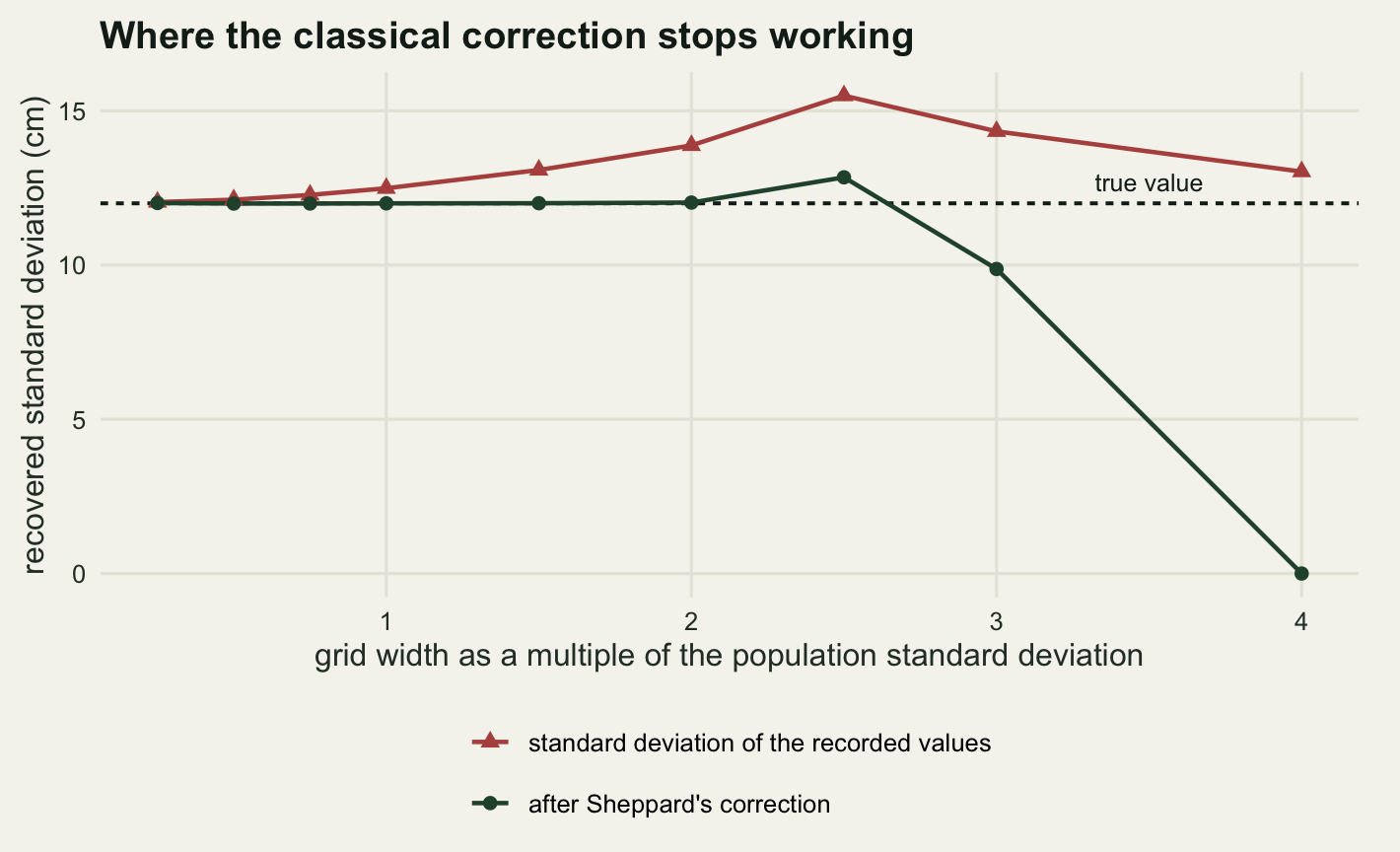
The correction is within five per cent of the measured inflation up to a grid of 2 times the population standard deviation, which covers every field grid worth arguing about: the heath’s 5 cm card is 0.4167 of a standard deviation. Past that it goes wrong in an order that surprised me. At 2.5 standard deviations the measured inflation is 1.2805 times the analytic value rather than less than it, so the correction under-subtracts and the recovered standard deviation comes out too high. Only at 3 does it swing the other way, to 9.8718 cm, and at 4 it subtracts more variance than the recorded values contain and returns 0. The clean uniform picture of the coarsening error is an approximation whose error terms oscillate, and by the time the grid is wider than the distribution there is no useful spread left in the recorded values to correct.
The mean survives, the shape does not
Now take one realisation of the scheme and look at what the grid did to it. Nothing here is resampled: these are the same seven hundred and twenty heights, read off a fine rule and then read off the card’s grid, and then off a much coarser grid for contrast.
set.seed(20260738)
z_heath <- rnorm(n_quad, mu_true, sd_true)
ht5 <- round_to(z_heath, h_card)
ht20 <- round_to(z_heath, 20)
print(c(distinct_exact = length(unique(z_heath)),
        distinct_5cm = length(unique(ht5)),
        distinct_20cm = length(unique(ht20))))
distinct_exact distinct_5cm distinct_20cm
720 17 5 print(round(c(mean_exact = mean(z_heath), mean_5cm = mean(ht5),
sd_exact = sd(z_heath), sd_5cm = sd(ht5),
sd_sheppard = sqrt(var(ht5) - h_card^2 / 12)), 4)) mean_exact mean_5cm sd_exact sd_5cm sd_sheppard
41.3402 41.3819 12.5309 12.6387 12.5560 p_exact <- shapiro.test(z_heath)$p.value
p_5cm <- shapiro.test(ht5)$p.value
p_20cm <- shapiro.test(ht20)$p.value
print(signif(c(shapiro_exact = p_exact, shapiro_5cm = p_5cm,
shapiro_20cm = p_20cm), 4))shapiro_exact shapiro_5cm shapiro_20cm
7.351e-01 2.012e-06 3.108e-27 The mean is essentially untouched: 41.3402 cm before rounding and 41.3819 after. The standard deviation moves the predicted amount and Sheppard puts it back, 12.556 against 12.5309. The Shapiro-Wilk test is a different story. On the exact heights it returns a p value of 0.7351, which is the correct answer, because the heights came out of rnorm. On the same heights read off the card’s grid it returns 2.01e-06, and on the coarse grid 3.11e-27. The population did not change, the sample did not change, and the ruler rejected normality at a level that would end any argument.
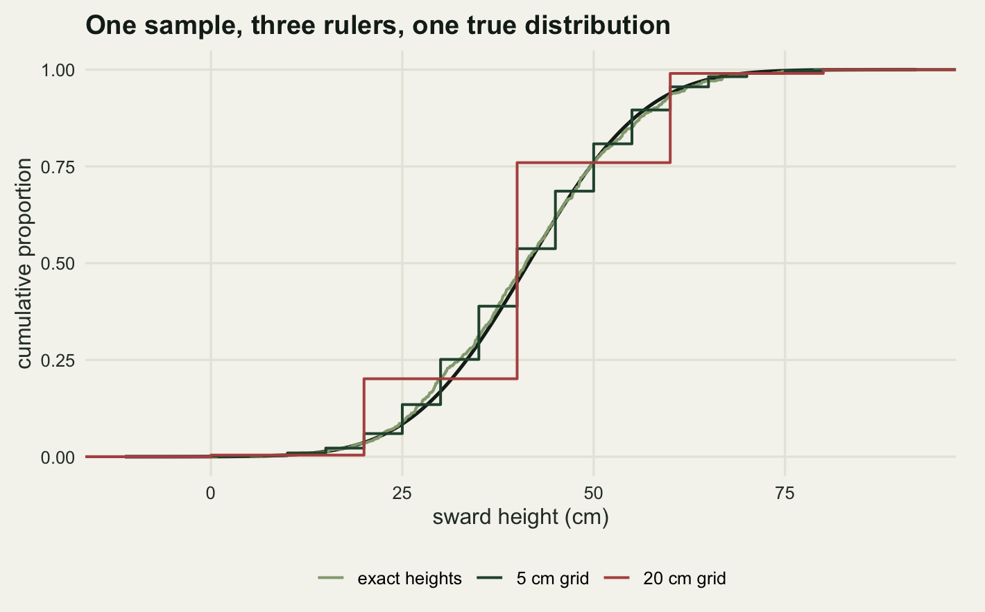
The staircase is the whole problem. A distributional test asks how far the empirical distribution is from the fitted one, and a step of width h is guaranteed to be half a tread away from a smooth curve through the middle of it. That distance does not shrink as the sample grows. It is a property of the ruler, so the test’s power against it goes to one and its verdict stops carrying information about the biology.
Making that concrete needs a rejection rate rather than a single p value, so the next chunk runs the test on data that are normal by construction and counts how often it says otherwise. The sample size is sixty, one site’s worth of quadrats, because a per-site normality check is the situation where this bites.
set.seed(20260734)
n_site <- 60
n_shape <- 3000
h_ladder <- c(0, 1, 2, 5, 10, 20)
shape_res <- do.call(rbind, lapply(h_ladder, function(h) {
  rej <- 0
  dis <- numeric(n_shape)
  for (r in seq_len(n_shape)) {
    z <- rnorm(n_site, mu_true, sd_true)
    y <- if (h == 0) z else round_to(z, h)
    dis[r] <- length(unique(y))
    p <- tryCatch(shapiro.test(y)$p.value, error = function(e) 0)
    if (p < 0.05) rej <- rej + 1
  }
  data.frame(h = h, distinct = mean(dis), sw_rej = rej / n_shape)
}))
print(round(shape_res, 4))
h distinct sw_rej
1 0 60.0000 0.0490
2 1 33.5613 0.0527
3 2 22.4653 0.0657
4 5 11.3130 0.2713
5 10 6.4743 1.0000
6 20 3.6337 1.0000rej_of <- function(h) shape_res$sw_rej[shape_res$h == h]
print(round(c(exact = rej_of(0), grid_5 = rej_of(5), grid_10 = rej_of(10),
grid_20 = rej_of(20)), 4)) exact grid_5 grid_10 grid_20
0.0490 0.2713 1.0000 1.0000 On exact draws the test rejects 4.9 per cent of the time, which is the nominal rate and confirms nothing is wrong with the setup. On the card’s five centimetre grid it rejects 27.13 per cent of the time, with an average of 11.31 distinct values among the sixty quadrats. On a ten centimetre grid it rejects 100 per cent and on twenty centimetres 100 per cent. Every one of those rejections is correct about the recorded values, which really are not normal, and useless about the population, which really is. The test is answering a question about the instrument.
The interval-censored likelihood, in three lines
The repair follows from what a recorded value means. A height written as 45 on a five centimetre grid says the true height was in the interval from 42.5 up to 47.5. That is a probability, not a density: the chance of an observation falling in a cell is the difference of the distribution function at the two edges. Write that down and maximise it. Heitjan (1989) reviews the general version, where an observation is known only up to an interval, a rectangle or some other region.
nll_ic <- function(par, y, h) {
  s <- exp(par[2])
  p <- pnorm(y + h / 2, par[1], s) - pnorm(y - h / 2, par[1], s)
  -sum(log(pmax(p, 1e-300)))
}

fit_ic <- function(y, h) {
  o <- optim(c(mean(y), log(max(sd(y), 1e-3))), nll_ic, y = y, h = h,
             method = "BFGS", hessian = TRUE)
  se <- sqrt(diag(solve(o$hessian)))
  c(mu = unname(o$par[1]), sigma = unname(exp(o$par[2])),
    se_mu = unname(se[1]), se_sigma = unname(exp(o$par[2]) * se[2]))
}

ic_heath <- fit_ic(ht5, h_card)
print(round(ic_heath, 4))
mu sigma se_mu se_sigma
41.3816 12.5471 0.4707 0.3350 print(round(c(exact_sample_mean = mean(z_heath), exact_sample_sd = sd(z_heath),
naive_sd = sd(ht5), sheppard_sd = sqrt(var(ht5) - h_card^2 / 12),
ic_sd = unname(ic_heath["sigma"])), 4))exact_sample_mean exact_sample_sd naive_sd sheppard_sd
41.3402 12.5309 12.6387 12.5560
ic_sd
12.5471 Against the heights the recorder never saw, the interval-censored fit returns a mean of 41.3816 cm with a standard error of 0.4707, and a standard deviation of 12.5471 with a standard error of 0.335. The exact sample values were 41.3402 and 12.5309. Sheppard’s correction gets to 12.556 by a different route and lands in the same place, which it should: Dempster and Rubin (1983) show the correction is what maximum likelihood reduces to when the grid is fine relative to the spread. The likelihood keeps working where the correction does not, and it comes with standard errors rather than a point estimate.
How well does it do on average, and is the interval it reports honest? The next chunk repeats the whole scheme several hundred times at three grid widths and records what each estimator returns, plus the coverage of the interval-censored confidence interval for the mean.
set.seed(20260737)
n_rec <- 800
rec_res <- do.call(rbind, lapply(c(5, 10, 20), function(h) {
  M <- matrix(NA_real_, n_rec, 5)
  for (r in seq_len(n_rec)) {
    y <- round_to(rnorm(n_quad, mu_true, sd_true), h)
    f <- fit_ic(y, h)
    M[r, ] <- c(mean(y), sd(y), sqrt(max(var(y) - h^2 / 12, 0)), f["sigma"],
                abs(f["mu"] - mu_true) < 1.96 * f["se_mu"])
  }
  data.frame(h = h, naive_mean = mean(M[, 1]), naive_sd = mean(M[, 2]),
             naive_excess_pct = 100 * (mean(M[, 2]) / sd_true - 1),
             sheppard_sd = mean(M[, 3]), ic_sd = mean(M[, 4]),
             ic_coverage = mean(M[, 5]))
}))
print(round(rec_res, 4))
h naive_mean naive_sd naive_excess_pct sheppard_sd ic_sd ic_coverage
1 5 41.4823 12.0827 0.6890 11.9961 11.9876 0.9663
2 10 41.5034 12.3338 2.7816 11.9909 11.9822 0.9362
3 20 41.5013 13.2712 10.5937 11.9484 11.9577 0.9388excess_of <- function(h) rec_res$naive_excess_pct[rec_res$h == h]The naive standard deviation is 0.689 per cent high on the five centimetre grid, 2.782 per cent on ten and 10.594 per cent on twenty. Both repairs remove almost all of it: at the coarsest grid Sheppard returns 11.9484 and the likelihood 11.9577 against a truth of 12. The interval for the mean covers the truth 96.63 per cent of the time on the fine grid and 93.88 per cent on the coarsest, a little under nominal at the coarse end but not by an amount that changes how a result would be read.
That leaves the goodness-of-fit problem, and the same idea fixes it. The recorded values are multinomial over the grid cells, with cell probabilities given by the differences of the fitted distribution function, so the natural test is a Pearson statistic on those cells rather than a test built for continuous data. Because the interval-censored fit is the grouped-data maximum likelihood estimate, the statistic keeps its usual chi-square reference distribution, with two degrees of freedom spent on the estimated parameters.
gof_grid <- function(y, h, mu, s, min_exp = 5) {
  lv <- seq(min(y), max(y), by = h)
  ob <- as.integer(table(factor(y, levels = lv)))
  edge_lo <- lv - h / 2
  edge_hi <- lv + h / 2
  edge_lo[1] <- -Inf
  edge_hi[length(edge_hi)] <- Inf
  ex <- length(y) * (pnorm(edge_hi, mu, s) - pnorm(edge_lo, mu, s))
  repeat {
    k <- length(ex)
    if (k <= 4) break
    i <- which.min(ex)
    if (ex[i] >= min_exp) break
    j <- if (i == 1) 2 else if (i == k) k - 1 else if (ex[i - 1] < ex[i + 1]) i - 1 else i + 1
    keep <- min(i, j)
    drop_at <- max(i, j)
    ob[keep] <- ob[i] + ob[j]
    ex[keep] <- ex[i] + ex[j]
    ob <- ob[-drop_at]
    ex <- ex[-drop_at]
  }
  dfree <- length(ex) - 3
  if (dfree < 1) return(c(x2 = NA_real_, dfree = NA_real_, p = NA_real_))
  x2 <- sum((ob - ex)^2 / ex)
  c(x2 = x2, dfree = dfree, p = pchisq(x2, dfree, lower.tail = FALSE))
}

gof_heath <- gof_grid(ht5, h_card, ic_heath["mu"], ic_heath["sigma"])
print(round(gof_heath, 4))
x2 dfree p
3.6410 10.0000 0.9621 set.seed(20260736)
n_gof <- 3000
gof_res <- do.call(rbind, lapply(c(1, 2, 5, 10, 20), function(h) {
rj <- 0
nv <- 0
for (r in seq_len(n_gof)) {
y <- round_to(rnorm(n_site, mu_true, sd_true), h)
f <- fit_ic(y, h)
p <- gof_grid(y, h, f["mu"], f["sigma"])["p"]
if (!is.na(p)) {
nv <- nv + 1
if (p < 0.05) rj <- rj + 1
}
}
data.frame(h = h, gof_rej = rj / nv, testable = nv / n_gof)
}))
print(round(gof_res, 4)) h gof_rej testable
1 1 0.0550 1.0000
2 2 0.0560 1.0000
3 5 0.0560 1.0000
4 10 0.0657 1.0000
5 20 0.1096 0.5443gof_of <- function(h) gof_res$gof_rej[gof_res$h == h]On the scheme’s own data the grid chi-square returns a p value of 0.9621 on 10 degrees of freedom, where Shapiro-Wilk on the same numbers returned 2.01e-06. Across three thousand replicates of a site the rejection rate holds near nominal: 5.5 per cent on a one centimetre grid, 5.6 per cent on five and 6.57 per cent on ten, against Shapiro-Wilk’s 100 per cent at that last grid.
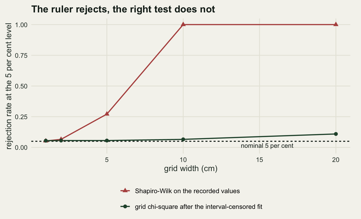
At twenty centimetres the grid test rises to 10.96 per cent, and the reason is in the last column of the table: only 54.4 per cent of replicates have enough occupied cells to test at all after pooling. With sixty quadrats spread over three or four distinct values there is almost nothing left to check, and the chi-square approximation is working on cells too thin to support it. That is a real limit of the repair rather than a failure of it: a test that cannot run is more honest than one that always rejects.
Distance sampling, where the claim was already on the site
Distance sampling for density in R closes with a list of conditions and one of them says that when distances are heaped at round numbers, binning the data into distance intervals helps. That is correct and it was never measured. Here is the measurement, on the same survey the post built: a thirty kilometre line, a truncation width of one hundred and fifty metres, a half-normal detection function with a scale of sixty metres, and a true density of eighty animals per square kilometre.
Three estimates of the same survey. Fit the detection function to the exact perpendicular distances, which is the analysis the original post ran. Fit it to distances rounded to a grid, which is the analysis anyone actually runs, because a perpendicular distance to a bird is estimated by eye and written down at the nearest twenty five or fifty metres. And fit it to the rounded distances treated as intervals, with the cells clipped at the line and at the truncation, because an animal recorded at zero was somewhere between the line and half a grid out, not on the line. The third of those is what the standard software calls binned or grouped distance data and will fit for you (Thomas et al. 2010; the design side is in Buckland et al. 2001); the point of building it by hand is to see the size of what it recovers.
d_true <- 80
len_line <- 30
w_tr <- 0.15
sig_true <- 0.06

g_area <- function(a, b, s) s * sqrt(2 * pi) * (pnorm(b / s) - pnorm(a / s))
esw_hn <- function(s) g_area(0, w_tr, s)
lo_b <- log(0.004)
hi_b <- log(2)

fit_point <- function(x) {
  nll <- function(ls) {
    s <- exp(ls)
    -sum(-x^2 / (2 * s^2) - log(esw_hn(s)))
  }
  exp(optim(lo_b, nll, method = "Brent", lower = lo_b, upper = hi_b)$par)
}

fit_interval <- function(y, h) {
  cell_lo <- pmax(y - h / 2, 0)
  cell_hi <- pmin(y + h / 2, w_tr)
  nll <- function(ls) {
    s <- exp(ls)
    -sum(log(pmax(g_area(cell_lo, cell_hi, s), 1e-300)) - log(esw_hn(s)))
  }
  exp(optim(lo_b, nll, method = "Brent", lower = lo_b, upper = hi_b)$par)
}

draw_survey <- function() {
  n_all <- round(d_true * 2 * w_tr * len_line)
  x_all <- runif(n_all, 0, w_tr)
  x_all[rbinom(n_all, 1, exp(-x_all^2 / (2 * sig_true^2))) == 1]
}

set.seed(20260741)
h_ds <- 0.05
x_ex <- draw_survey()
x_rd <- pmin(round_to(x_ex, h_ds), w_tr)
s_ex <- fit_point(x_ex)
s_rd <- fit_point(x_rd)
s_iv <- fit_interval(x_rd, h_ds)
dens_from <- function(s) length(x_ex) / (2 * len_line * esw_hn(s))
one_survey <- c(n_detected = length(x_ex), sigma_exact = s_ex,
                sigma_rounded = s_rd, sigma_interval = s_iv,
                esw_exact = esw_hn(s_ex), esw_rounded = esw_hn(s_rd),
                esw_interval = esw_hn(s_iv), d_exact = dens_from(s_ex),
                d_rounded = dens_from(s_rd), d_interval = dens_from(s_iv))
print(round(one_survey, 4))
n_detected sigma_exact sigma_rounded sigma_interval esw_exact
355.0000 0.0607 0.0629 0.0602 0.0750
esw_rounded esw_interval d_exact d_rounded d_interval
0.0775 0.0744 78.8789 76.3079 79.4732 One survey detected 355 animals. On the exact distances the effective strip half-width comes out at 0.075 km and the density at 78.88 animals per square kilometre against a truth of 80. Round every distance to the nearest fifty metres and the same detections give an effective strip half-width of 0.0775 km, which is wider, and a density of 76.31, which is lower. Treat the rounded values as the intervals they are and the density returns to 79.47.
One survey is one draw, so the direction of that shift needs a few hundred more of them, at several grid widths.
set.seed(20260742)
n_ds <- 400
ds_res <- do.call(rbind, lapply(c(0.01, 0.025, 0.05, 0.075), function(h) {
  M <- matrix(NA_real_, n_ds, 4)
  for (r in seq_len(n_ds)) {
    xx <- draw_survey()
    yy <- pmin(round_to(xx, h), w_tr)
    M[r, ] <- c(length(xx) / (2 * len_line * esw_hn(fit_point(xx))),
                length(xx) / (2 * len_line * esw_hn(fit_point(yy))),
                length(xx) / (2 * len_line * esw_hn(fit_interval(yy, h))),
                mean(yy^2) - mean(xx^2))
  }
  data.frame(grid_m = h * 1000, d_exact = mean(M[, 1]), d_rounded = mean(M[, 2]),
             d_interval = mean(M[, 3]),
             rounded_pct = 100 * (mean(M[, 2]) / d_true - 1),
             interval_pct = 100 * (mean(M[, 3]) / d_true - 1),
             moment_shift = mean(M[, 4]),
             moment_ratio = mean(M[, 4]) / (h^2 / 12))
}))
print(round(ds_res, 4))
grid_m d_exact d_rounded d_interval rounded_pct interval_pct moment_shift
1 10 80.0830 79.9443 80.0788 -0.0696 0.0985 0e+00
2 25 80.0508 79.1868 80.0306 -1.0164 0.0382 1e-04
3 50 80.4598 77.1398 80.4476 -3.5753 0.5595 2e-04
4 75 79.7229 72.6338 79.6384 -9.2078 -0.4520 5e-04
moment_ratio
1 1.1084
2 1.1166
3 1.0971
4 1.0997ds_res$grid_over_scale <- ds_res$grid_m / (sig_true * 1000)
pct_at <- function(g) ds_res$rounded_pct[ds_res$grid_m == g]
iv_at <- function(g) ds_res$interval_pct[ds_res$grid_m == g]
ratio_at <- function(g) ds_res$grid_over_scale[ds_res$grid_m == g]
print(round(ds_res[, c("grid_m", "grid_over_scale", "rounded_pct", "interval_pct")], 4)) grid_m grid_over_scale rounded_pct interval_pct
1 10 0.1667 -0.0696 0.0985
2 25 0.4167 -1.0164 0.0382
3 50 0.8333 -3.5753 0.5595
4 75 1.2500 -9.2078 -0.4520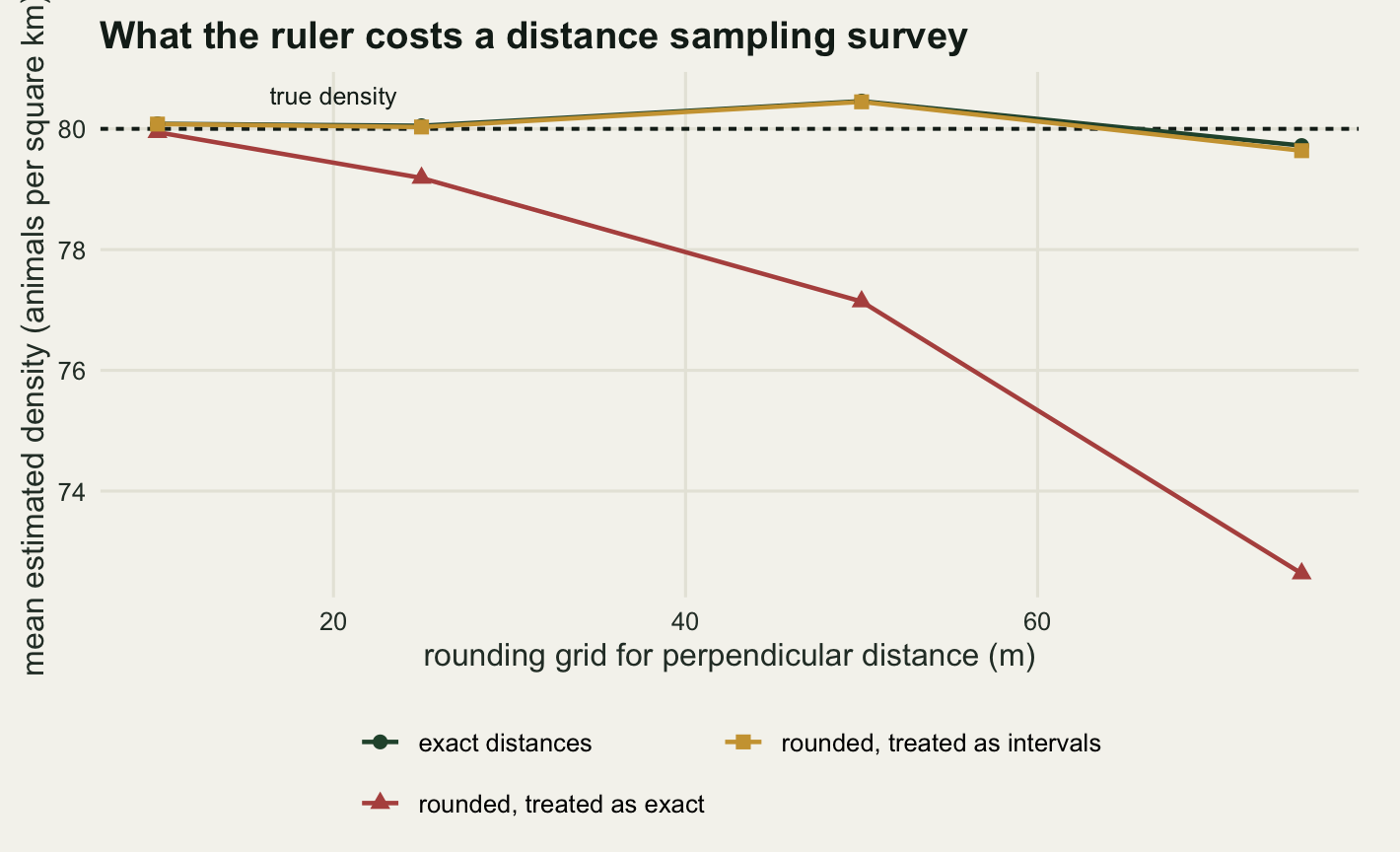
Rounding to the nearest ten metres costs 0.07 per cent of the density, which is nothing next to the sampling error of a single survey. At twenty five metres it is 1.016 per cent, at fifty 3.575 per cent and at seventy five 9.208 per cent, all in the same direction, all towards fewer animals. The interval-censored fit is within 0.559 per cent of the truth at every grid tried. So the original post’s advice holds, with a size attached to it. What sets the size is the grid measured against the detection scale: at 0.167 of the scale the loss is under a tenth of a per cent and the repair is not worth the code, at 0.417 it is about one per cent, and once the grid reaches 1.25 times the scale it takes most of a tenth off the density.
The mechanism is the one from the first section, wearing different clothes. The half-normal likelihood depends on the distances only through their sum of squares, so anything that inflates the second moment inflates the fitted scale, widens the effective strip and divides the count by too large a number.
print(round(ds_res[, c("grid_m", "moment_shift", "moment_ratio")], 6)) grid_m moment_shift moment_ratio
1 10 0.000009 1.108435
2 25 0.000058 1.116566
3 50 0.000229 1.097058
4 75 0.000515 1.099697mom_lo <- min(ds_res$moment_ratio)
mom_hi <- max(ds_res$moment_ratio)The second moment of the recorded distances exceeds the second moment of the true distances by between 1.097 and 1.117 times h squared over twelve at every grid width tried. It is Sheppard’s term again, arriving inside the sufficient statistic of a detection function instead of inside a sample variance, and the excess over one is the truncation: a cell at the edge of the strip is clipped, so the coarsening error there is not symmetric.
What has to be true about the grid
Everything above assumes the grid is known, regular and the same for every observation. Drop any of the three and the likelihood needs more information than the field sheet holds.
The common failure is a mixed grid. Half the recorders in the scheme use the card’s five centimetre marks and half work to the nearest twenty, and the data come back in one column with nothing to say which is which.
nll_mix <- function(par, y, hv) {
  s <- exp(par[2])
  -sum(log(pmax(pnorm(y + hv / 2, par[1], s) - pnorm(y - hv / 2, par[1], s), 1e-300)))
}
fit_mix <- function(y, hv) {
  o <- optim(c(mean(y), log(sd(y))), nll_mix, y = y, hv = hv, method = "BFGS")
  c(mu = unname(o$par[1]), sigma = unname(exp(o$par[2])))
}

set.seed(20260743)
n_mix <- 400
M_mix <- t(replicate(n_mix, {
  z <- rnorm(n_quad, mu_true, sd_true)
  hv <- rep(c(h_card, 20), each = n_quad / 2)
  y <- round_to(z, hv)
  c(sd(y), fit_mix(y, rep(h_card, n_quad))["sigma"],
    fit_mix(y, rep(20, n_quad))["sigma"], fit_mix(y, hv)["sigma"])
}))
mix_res <- c(naive_sd = mean(M_mix[, 1]), assume_fine = mean(M_mix[, 2]),
             assume_coarse = mean(M_mix[, 3]), per_observation = mean(M_mix[, 4]))
print(round(mix_res, 4))
naive_sd assume_fine assume_coarse per_observation
12.6875 12.5962 11.3067 11.9679 print(round(100 * (mix_res / sd_true - 1), 3)) naive_sd assume_fine assume_coarse per_observation
5.729 4.968 -5.777 -0.268 Assuming everyone used the fine grid returns a standard deviation of 12.5962, which is 4.968 per cent high because it never subtracts the coarse recorders’ extra spread. Assuming everyone used the coarse grid returns 11.3067, 5.777 per cent low, because it subtracts spread the fine recorders never added. Give the likelihood one interval per observation and it returns 11.9679, within 0.268 per cent of the truth. The code change is trivial: h becomes a vector. The data change is not, because the vector has to come from somewhere, and if the field sheet does not record who measured which quadrat, that information does not exist any more.
The same problem arrives in a second form when the grid varies with the measurement. A distance of eight metres gets written as 8; a distance of two hundred gets written as 200 rather than 197, because precision falls off with range. The grid is then a function of the value, the cells are unequal, and the interval per observation has to be built from a rule about the observer’s behaviour rather than read off the card. Marques (2004) treats exactly this for line transects by modelling the error multiplicatively, which is the right shape when the resolution scales with the distance.
Two smaller conditions are worth stating. The cell edges have to be where you think they are: a recorder who truncates rather than rounds, writing 35 for anything from 35 up to 40, puts the interval at the wrong place and the fitted mean will be half a grid out. And the underlying distribution has to be smooth across a cell, which is what fails at the coarse end of the sweep above. Heitjan and Rubin (1991) give the general condition under which the coarsening can be ignored in the likelihood; the useful summary is that the grid may depend on anything you are conditioning on, and must not depend on the unobserved true value in a way you cannot write down.
What to take away
The number on the field card is a cell label, not a measurement, and treating it as a measurement has a cost that can be written down in advance. Rounding to a grid of width h adds h squared over twelve to the variance: measured at 2.116 against a predicted 2.0833 on the heath scheme’s grid, a ratio of 1.0157, and Sheppard’s correction takes it back out to within 0.0067 per cent of the truth. That correction stays good up to a grid of 2 population standard deviations and then fails in both directions.
The mean is not the problem. Across two thousand realisations the rounded mean sat -0.01552 cm from the truth with a Monte Carlo standard error of 0.01003, so there is nothing there to correct. The shape is the problem. On draws that were normal by construction, Shapiro-Wilk rejected normality 27.13 per cent of the time on a five centimetre grid and 100 per cent on a ten centimetre one. Nothing biological changed between those two rates. The ruler did.
Writing the likelihood on intervals instead of points fixes both halves. It recovered the standard deviation to 11.9577 against 12 on a twenty centimetre grid where the naive estimate was 10.594 per cent high, and the matching goodness-of-fit test on the grid cells held its rejection rate at 5.6 per cent where Shapiro-Wilk was at 27.13 per cent. In the distance-sampling survey it recovered a density biased 3.575 per cent low at a fifty metre grid to within 0.559 per cent of the truth.
Two results came out other than expected. Sheppard’s correction does not degrade gracefully: at a grid of two and a half standard deviations the measured inflation is 1.2805 times the analytic value, so the correction under-subtracts and the answer is too high, before turning over and collapsing to 0 at four. And the grid chi-square, which holds its nominal rate everywhere else, drifts to 10.96 per cent at the coarsest grid, where only 54.4 per cent of samples have enough occupied cells to test.
The honest limit is that none of this is recoverable from the numbers alone. The likelihood needs one interval per observation, and the intervals come from knowing the grid: which recorder, which instrument, whether they rounded or truncated, whether the resolution changed with the size of the thing being measured. That is metadata, it lives on the field sheet or nowhere, and a column of numbers that all end in 0 or 5 tells you a grid was used without telling you which one. The cheapest useful habit is therefore not a correction at all. It is a column on the recording form for the resolution actually used, filled in once per recorder per visit, which costs a second in the field and is the difference between an exact likelihood and a guess.
References
Sheppard WF 1897 Proceedings of the London Mathematical Society s1-29(1):353-380 (10.1112/plms/s1-29.1.353)
Dempster AP, Rubin DB 1983 Journal of the Royal Statistical Society Series B 45(1):51-59 (10.1111/j.2517-6161.1983.tb01230.x)
Vardeman SB 2005 IEEE Transactions on Instrumentation and Measurement 54(5):2117-2119 (10.1109/TIM.2005.853348)
Heitjan DF 1989 Statistical Science 4(2):164-179 (10.1214/ss/1177012601)
Heitjan DF, Rubin DB 1991 The Annals of Statistics 19(4):2244-2253 (10.1214/aos/1176348396)
Marques TA 2004 Biometrics 60(3):757-763 (10.1111/j.0006-341X.2004.00226.x)
Thomas L, Buckland ST, Rexstad EA, Laake JL, Strindberg S, Hedley SL, Bishop JRB, Marques TA, Burnham KP 2010 Journal of Applied Ecology 47(1):5-14 (10.1111/j.1365-2664.2009.01737.x)
Stewart KEJ, Bourn NAD, Thomas JA 2001 Journal of Applied Ecology 38(5):1148-1154 (10.1046/j.1365-2664.2001.00658.x)
Buckland ST, Anderson DR, Burnham KP, Laake JL, Borchers DL, Thomas L 2001 Introduction to Distance Sampling (Oxford University Press, ISBN 978-0-19-850927-1)