---
title: "Dichotomising a continuous confounder"
description: "Splitting a continuous confounder at its median leaves part of it unadjusted, so a null predictor can turn significant in ecological surveys. Measured in R."
date: "2026-08-10 14:00"
categories: [R, causal inference, regression, simulation, ecology tutorial]
image: thumbnail.png
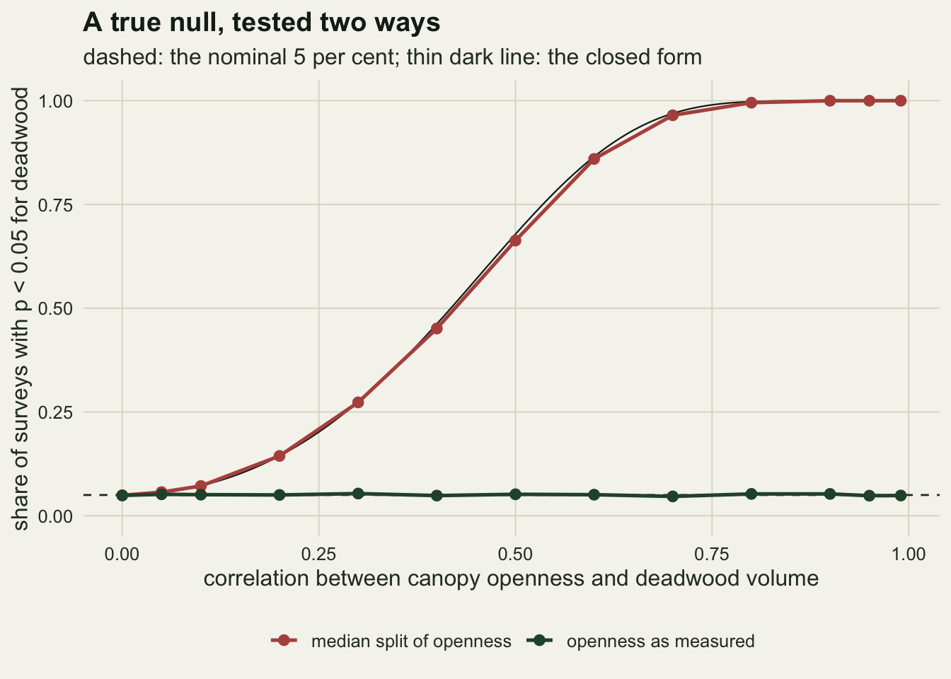
image-alt: "A line chart on warm off-white paper, headed a true null tested two ways. The horizontal axis is the correlation between the confounder and the predictor, from zero to one; the vertical axis is the share of surveys with a p value below five hundredths. A red line for the median split climbs from five per cent at zero correlation to one hundred per cent by a correlation of nine tenths, while a green line for the confounder as measured stays flat along a dashed reference line at five per cent."
---
A regeneration survey covers two hundred plots of a hundred square metres each in a mixed broadleaf forest. Every plot carries a hemispherical photograph, which gives canopy openness as a percentage of visible sky, a tally of fallen stems converted to a deadwood volume per hectare, and a count of tree seedlings taller than twenty centimetres. The question is whether deadwood helps regeneration: fallen stems hold moisture, and a lattice of coarse wood keeps deer off the seedlings growing beside it.
Canopy openness has to be in the model. It drives recruitment through light, and it is correlated with deadwood volume for an obvious reason: both are made by a tree coming down. It is a confounder in the plain sense, and it was measured well, on a continuous scale, in every plot.
What usually happens next is the subject of this post. Openness gets cut at its median and the halves are labelled closed and open, because a two-level factor plots cleanly, reads cleanly in a table, and matches the way foresters already talk about gaps. The cut is not presented as a modelling decision at all. It is presented as a description.
This post runs that survey several thousand times with the deadwood effect set to exactly zero, and measures what the cut costs. The result is not that the split loses the confounder's effect on recruitment; it keeps most of that. The split loses the confounder's linear association with the predictor of interest, and the two are different quantities with different consequences. That is also what separates this from its neighbours on the site: [measurement error](../measurement-error-regression-dilution/) flags that a noisy covariate contaminates the coefficients of well-measured ones, and this post is the measurement of that flag for a covariate carrying no noise at all, coarsened on purpose; [baseline selection](../baseline-selection-and-the-return-to-mean/) covers additive noise on a repeated baseline, where the leak is a reliability ratio rather than a constant; and [unmeasured confounding](../sensitivity-to-unmeasured-confounding/) is about a covariate you never had, whereas here the covariate is in hand, in the model, and the adjustment set is right.
## One survey, two ways to hold openness fixed
The generating process below is the survey as described, standardised: openness and deadwood volume are correlated, openness drives recruitment, and deadwood does nothing whatsoever.
```{r setup}
#| message: false
#| warning: false
library(ggplot2)
library(patchwork)

te_paper  <- "#f5f4ee"
te_ink    <- "#16241d"
te_body   <- "#2c3a31"
te_forest <- "#275139"
te_rust   <- "#b5534e"
te_line   <- "#dad9ca"

theme_datasheet <- function() {
  theme_minimal(base_size = 12) +
    theme(plot.background  = element_rect(fill = te_paper, colour = NA),
          panel.background = element_rect(fill = te_paper, colour = NA),
          panel.grid.major = element_line(colour = te_line, linewidth = 0.3),
          panel.grid.minor = element_blank(),
          text             = element_text(colour = te_body),
          plot.title       = element_text(colour = te_ink, face = "bold"),
          plot.subtitle    = element_text(colour = te_body),
          axis.text        = element_text(colour = te_body))
}

n_plot   <- 200
rho_base <- 0.6
b_open   <- 1
sde_base <- 1

set.seed(1)
openness <- rnorm(n_plot)
deadwood <- rho_base * openness + sqrt(1 - rho_base^2) * rnorm(n_plot)
one <- data.frame(openness, deadwood,
                  recruit = b_open * openness + rnorm(n_plot, 0, sde_base),
                  open_class = ifelse(openness > median(openness), "open", "closed"))

fit_cont  <- lm(recruit ~ deadwood + openness, data = one)
fit_split <- lm(recruit ~ deadwood + open_class, data = one)

coef_cont  <- summary(fit_cont)$coefficients["deadwood", ]
coef_split <- summary(fit_split)$coefficients["deadwood", ]
round(rbind(as_measured = coef_cont, median_split = coef_split), 4)
```
With openness in the model as measured, the deadwood coefficient is `r sprintf("%.3f", coef_cont[1])` with a p value of `r sprintf("%.2f", coef_cont[4])`, which is the correct answer: there is no deadwood effect in the generator. With openness in the model as two classes, the same survey returns `r sprintf("%.3f", coef_split[1])` and a p value of `r sprintf("%.4f", coef_split[4])`. Nothing was dropped, nothing was mismeasured, and the adjustment set was not changed. One covariate was described in two classes instead of one number. That is a single draw, the first seed tried, and a single draw proves nothing. The rest of the post asks how often it comes out that way, and why.
## The null is true and the split rejects it anyway
Sweep the correlation between openness and deadwood from zero to nearly one, and at each value run the survey several thousand times under each adjustment. The deadwood effect stays at zero throughout, so every rejection is a false positive.
```{r rhosweep}
leak_q <- function(q) {
  z <- qnorm(q)
  1 - dnorm(z)^2 / (q * (1 - q))
}
rej_closed <- function(n, rho, b1, sde, k) {
  v_res <- 1 - rho^2 * (1 - k)
  ncp   <- (b1 * rho * k / v_res) *
    sqrt(n * v_res / (sde^2 + b1^2 * (k - rho^2 * k^2 / v_res)))
  crit <- qt(0.975, n - 3)
  pt(-crit, n - 3, ncp) + pt(-crit, n - 3, -ncp)
}

sim_cell <- function(nsim, n, rho, b1, sde, adj, q = 0.5, dep = "linear", seed) {
  set.seed(seed)
  n_rej <- 0
  est <- numeric(nsim)
  for (i in seq_len(nsim)) {
    openness <- rnorm(n)
    deadwood <- if (dep == "linear") rho * openness + sqrt(1 - rho^2) * rnorm(n) else
      scale(rho * (openness^2 - 1) / sqrt(2) + sqrt(1 - rho^2) * rnorm(n))[, 1]
    recruit  <- b1 * openness + rnorm(n, 0, sde)
    adj_mat <- if (adj == "cont") cbind(openness) else if (adj == "split") {
      cbind(as.numeric(openness > quantile(openness, q)))
    } else {
      edge <- quantile(openness, seq(0, 1, length.out = as.integer(adj) + 1))
      model.matrix(~ 0 + cut(openness, edge, include.lowest = TRUE))[, -1, drop = FALSE]
    }
    design <- cbind(1, deadwood, adj_mat)
    fit <- .lm.fit(design, recruit)
    np <- ncol(design)
    s2 <- sum(fit$residuals^2) / (n - np)
    vv <- chol2inv(chol(crossprod(design)))[2, 2]
    n_rej <- n_rej + (abs(fit$coefficients[2] / sqrt(s2 * vv)) > qt(0.975, n - np))
    est[i] <- fit$coefficients[2]
  }
  pr <- n_rej / nsim
  data.frame(adj, n, rho, sde, q, rej = pr, se_rej = sqrt(pr * (1 - pr) / nsim),
             bias = mean(est), se_bias = sd(est) / sqrt(nsim))
}

nsim_rho <- 8000
rho_grid <- c(0, 0.05, 0.1, 0.2, 0.3, 0.4, 0.5, 0.6, 0.7, 0.8, 0.9, 0.95, 0.99)

sweep_split <- do.call(rbind, lapply(seq_along(rho_grid), function(i)
  sim_cell(nsim_rho, n_plot, rho_grid[i], b_open, sde_base, "split", seed = 300 + i)))
sweep_cont <- do.call(rbind, lapply(seq_along(rho_grid), function(i)
  sim_cell(nsim_rho, n_plot, rho_grid[i], b_open, sde_base, "cont", seed = 300 + i)))

at_base  <- which(rho_grid == rho_base)
at_zero  <- which(rho_grid == 0)
at_high  <- which(rho_grid == 0.9)
at_max   <- which(rho_grid == 0.99)
rej_split_base <- sweep_split$rej[at_base]
rej_cont_base  <- sweep_cont$rej[at_base]
bias_base      <- sweep_split$bias[at_base]
```
At a correlation of `r sprintf("%.1f", rho_base)`, the split-adjusted analysis reports a significant deadwood effect in `r sprintf("%.1f", 100 * rej_split_base)` per cent of `r sprintf("%d", nsim_rho)` surveys, with a Monte Carlo standard error of `r sprintf("%.1f", 100 * sweep_split$se_rej[at_base])` percentage points. The two sweeps share their seeds, so those are the same surveys analysed a second way: with openness as measured they reject in `r sprintf("%.1f", 100 * rej_cont_base)` per cent of cases, which is the level the test advertises. The average deadwood coefficient under the split is `r sprintf("%.4f", bias_base)` against a truth of zero, so this is a shifted estimate and not a widened one. Both ends of the sweep behave. With openness and deadwood uncorrelated the split is harmless: `r sprintf("%.4f", sweep_split$rej[at_zero])` under the split against `r sprintf("%.4f", sweep_cont$rej[at_zero])` as measured. At the other end the split rejects in every one of the surveys once the correlation reaches `r sprintf("%.1f", rho_grid[at_high])`, while the continuous adjustment is still at `r sprintf("%.4f", sweep_cont$rej[at_max])` when the correlation is `r sprintf("%.2f", rho_grid[at_max])`, so none of this is collinearity.
```{r figsweep}
#| fig-cap: "False-positive rate against the openness to deadwood correlation, under two adjustments, with the closed-form prediction overlaid."
#| fig-alt: "A line chart with correlation from zero to one on the horizontal axis and the share of surveys reporting a significant deadwood effect on the vertical axis. The red median-split series starts at five per cent, rises past fifty per cent between correlations of four tenths and one half, and flattens at one hundred per cent from nine tenths onwards. The green series for openness as measured runs flat along the dashed five per cent reference line across the whole range. A thin dark line tracks the red series closely."
sweep_long <- data.frame(rho = rho_grid, rej = c(sweep_split$rej, sweep_cont$rej),
  adjustment = rep(c("median split of openness", "openness as measured"), each = length(rho_grid)))
closed_line <- data.frame(rho = seq(0, 0.99, length.out = 200))
closed_line$rej <- rej_closed(n_plot, closed_line$rho, b_open, sde_base, leak_q(0.5))

ggplot(sweep_long, aes(rho, rej, colour = adjustment)) +
  geom_line(data = closed_line, aes(rho, rej), inherit.aes = FALSE,
            colour = te_ink, linewidth = 0.4) +
  geom_hline(yintercept = 0.05, linetype = "dashed", colour = te_body, linewidth = 0.5) +
  geom_line(linewidth = 0.9) +
  geom_point(size = 2.2) +
  scale_colour_manual(values = c(te_rust, te_forest), name = NULL) +
  scale_y_continuous(limits = c(0, 1)) +
  labs(x = "correlation between canopy openness and deadwood volume",
       y = "share of surveys with p < 0.05 for deadwood",
       title = "A true null, tested two ways",
       subtitle = "dashed: the nominal 5 per cent; thin dark line: the closed form") +
  theme_datasheet() +
  theme(legend.position = "bottom")
```
## What the split loses is over a third of the openness axis, and that is algebra
The thin dark line in the figure is not a fit. It is the exact asymptotic rate for a cut placed at the known population median, which is not what the simulation does: there the cut is the sample median, re-estimated in every survey. The line sits a little above the points through the middle of the range rather than on them, and that difference between a known cut and an estimated one is the likely reason. It is worth writing out because it names the quantity that does the damage.
Let openness be standard normal and let `D` be the indicator that it exceeds its median. Then the correlation between the variable and its own indicator is `sqrt(2/pi)`, the indicator explains `2/pi` of the variance of openness, and what is left over is
`k = 1 - 2/pi`
the share of the openness axis that stays in the error term after the two classes have been fitted. This `k` is a fraction of variance, not a fraction of an effect and not a correlation, and getting that noun right is the difference between the correct account and a plausible wrong one. Write the openness axis as a class effect plus a remainder, and the remainder has variance `k`. The class effect is adjusted for. The remainder is not, and it is still correlated with deadwood volume, which is what makes it dangerous rather than merely wasteful. Becher (1992) sets out the same decomposition for categorised confounders in epidemiology.
```{r leak}
k_median <- 1 - 2 / pi

set.seed(5)
n_check <- 4e6
leak_measured <- function(x) 1 - cor(x, as.numeric(x > median(x)))^2

k_normal <- leak_measured(rnorm(n_check))
k_unif   <- leak_measured(runif(n_check))
k_lnorm  <- leak_measured(rlnorm(n_check))
k_expo   <- leak_measured(rexp(n_check))
k_t3     <- leak_measured(rt(n_check, 3))

k_unif_exact  <- 1 - 3 / 4
k_expo_exact  <- 1 - log(2)^2
k_lnorm_exact <- 1 - ((exp(0.5) * pnorm(1) - exp(0.5) / 2) /
                        (sqrt(exp(2) - exp(1)) * 0.5))^2
exact_gap <- max(abs(c(k_unif - k_unif_exact, k_expo - k_expo_exact,
                       k_lnorm - k_lnorm_exact)))
bias_closed <- b_open * rho_base * k_median / (1 - rho_base^2 * (1 - k_median))
round(c(normal = k_normal, uniform = k_unif, exponential = k_expo,
        t_3df = k_t3, lognormal = k_lnorm), 4)
```
Simulating four million draws returns `r sprintf("%.4f", k_normal)` against the algebraic `r sprintf("%.6f", k_median)`, which is a check on the machinery rather than a discovery. The same is true of the bias itself. With `b` for the openness effect on recruitment and `rho` for the openness to deadwood correlation, the deadwood coefficient converges on
`b * rho * k / (1 - rho^2 * (1 - k))`
and at the base design that is `r sprintf("%.4f", bias_closed)` against a simulated `r sprintf("%.4f", bias_base)`. Everything the closed form claims is visible in the sweep, so the simulation is doing the job of confirming the arithmetic, not of finding something new. Austin and Brunner (2004) measured the same size distortion for categorised confounders in logistic regression.
The constant is a normality result, and the leak moves with the shape of the covariate in both directions. A uniform covariate cut at its median leaves `r sprintf("%.4f", k_unif)` unadjusted, an exponential one `r sprintf("%.4f", k_expo)` and a lognormal one `r sprintf("%.4f", k_lnorm)`. Each of those three has its own closed form, and the simulated values sit within `r sprintf("%.4f", exact_gap)` of it, so they are identities in the same sense the normal case is. The t distribution on three degrees of freedom has a closed form too, at `1 - 4/pi^2`, and its simulated `r sprintf("%.4f", k_t3)` sits a little further from that value than the other three sit from theirs: the distribution has no fourth moment, so its sample standard deviation settles slowly and the Monte Carlo error is larger. Deadwood volume, seed rain, distance to a source and nutrient concentration are all right skewed, and a lognormal confounder leaves roughly three quarters of itself in the residual.
## The bias is fixed and the rejection rate is a design choice
A false-positive rate of `r sprintf("%.1f", 100 * rej_split_base)` per cent is a property of that grid cell, not of dichotomising. Hold the correlation and the openness effect fixed and move the sample size, then move the residual noise.
```{r invariance}
n_grid <- c(50, 100, 500, 2000)
inv_n <- do.call(rbind, lapply(seq_along(n_grid), function(i)
  sim_cell(4000, n_grid[i], rho_base, b_open, sde_base, "split", seed = 520 + i)))

sde_grid <- c(0.25, 0.5, 2, 4)
inv_sde <- do.call(rbind, lapply(seq_along(sde_grid), function(i)
  sim_cell(4000, n_plot, rho_base, b_open, sde_grid[i], "split", seed = 610 + i)))

bias_span <- range(c(inv_n$bias, inv_sde$bias))
round(rbind(inv_n, inv_sde)[, c("n", "sde", "rej", "bias")], 4)
```
Across a fortyfold range of sample size the false-positive rate runs from `r sprintf("%.4f", round(inv_n$rej[1], 4))` at `r sprintf("%d", n_grid[1])` plots to `r sprintf("%.4f", inv_n$rej[4])` at `r sprintf("%d", n_grid[4])`, while the bias sits between `r sprintf("%.4f", bias_span[1])` and `r sprintf("%.4f", bias_span[2])` in every one of the eight cells. Sharpening the survey makes it worse, not better: cutting the residual noise to a quarter takes the rate to `r sprintf("%.4f", inv_sde$rej[1])`, and quadrupling it drops the rate to `r sprintf("%.4f", inv_sde$rej[4])` without touching the bias at all. The reason more data does not help is that this is a bias and not a variance problem. The estimate is converging, and it is converging on the wrong number, so the interval around it shrinks onto a value that is not zero and the test rejects with certainty in the limit. Quoting one rejection rate as the cost of a median split is therefore quoting the sample size, the effect of the confounder and the residual noise, all at once, without saying so.
## Getting the outcome shape right does not repair it
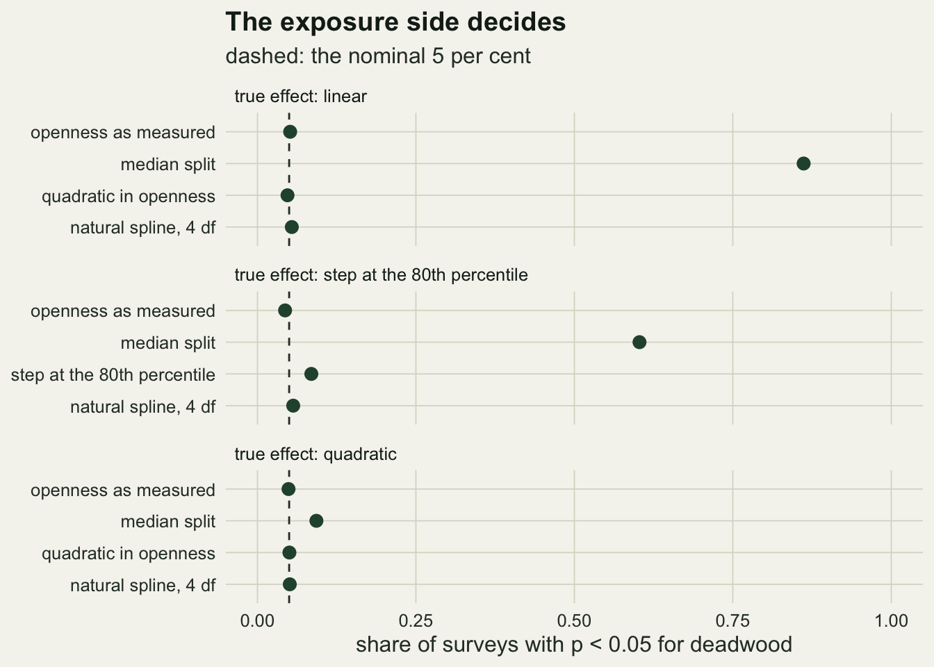
If the trouble were that a step function is a poor description of how openness drives recruitment, then modelling that relationship correctly would fix it. Cross the true shape of the openness effect against the shape used to adjust for it and the explanation fails.
```{r forms}
form_cell <- function(nsim, n, rho, sde, shape, adj, seed) {
  set.seed(seed)
  n_rej <- 0
  est <- numeric(nsim)
  for (i in seq_len(nsim)) {
    openness <- rnorm(n)
    deadwood <- rho * openness + sqrt(1 - rho^2) * rnorm(n)
    truth <- switch(shape, linear = openness, quad = openness^2,
                    step80 = as.numeric(openness > qnorm(0.8)))
    recruit <- scale(truth)[, 1] + rnorm(n, 0, sde)
    adj_mat <- switch(adj, cont = cbind(openness), spline = splines::ns(openness, 4),
                      split  = cbind(as.numeric(openness > median(openness))),
                      step80 = cbind(as.numeric(openness > quantile(openness, 0.8))),
                      quadratic = cbind(openness, openness^2))
    design <- cbind(1, deadwood, adj_mat)
    fit <- .lm.fit(design, recruit)
    np <- ncol(design)
    s2 <- sum(fit$residuals^2) / (n - np)
    vv <- chol2inv(chol(crossprod(design)))[2, 2]
    n_rej <- n_rej + (abs(fit$coefficients[2] / sqrt(s2 * vv)) > qt(0.975, n - np))
    est[i] <- fit$coefficients[2]
  }
  pr <- n_rej / nsim
  data.frame(shape, adj, rej = pr, se_rej = sqrt(pr * (1 - pr) / nsim),
             bias = mean(est), se_bias = sd(est) / sqrt(nsim))
}

form_grid <- rbind(
  c("linear", "cont"), c("linear", "split"), c("linear", "quadratic"), c("linear", "spline"),
  c("step80", "cont"), c("step80", "split"), c("step80", "step80"), c("step80", "spline"),
  c("quad", "cont"), c("quad", "split"), c("quad", "quadratic"), c("quad", "spline"))

forms <- do.call(rbind, lapply(seq_len(nrow(form_grid)), function(i)
  form_cell(5000, n_plot, rho_base, sde_base, form_grid[i, 1], form_grid[i, 2],
            seed = 900 + i)))

pick <- function(sh, ad) forms[forms$shape == sh & forms$adj == ad, ]
step_wrong <- pick("step80", "cont")
step_right <- pick("step80", "step80")
step_split <- pick("step80", "split")
step_spline <- pick("step80", "spline")
quad_split <- pick("quad", "split")
cbind(forms[, 1:2], round(forms[, 3:6], 4))
```
Take the middle block, where openness really does act as a step at its eightieth percentile: recruitment is one value in the gappiest fifth of plots and another value everywhere else. Adjusting for openness as a straight line is then a badly wrong description of the outcome, and it does not exceed the nominal level: `r sprintf("%.4f", step_wrong$rej)` with a standard error of `r sprintf("%.4f", step_wrong$se_rej)`. Adjusting with a step at the same percentile, the outcome model with the right shape by construction, gives `r sprintf("%.4f", step_right$rej)`, which is not nominal, and carries a bias of `r sprintf("%.4f", step_right$bias)`. The median split in the same block gives `r sprintf("%.4f", step_split$rej)`.
The ordering is the point. A wrong outcome shape with a covariate on its original scale is safe; a right outcome shape with the covariate coarsened is not. What the linear term does is remove the part of openness that predicts deadwood, and under joint normality the deadwood residual is then independent of openness, so whatever shape is left in the recruitment residual cannot correlate with it. What the step does is leave `k` of the openness axis behind, still correlated with deadwood, no matter how well it describes recruitment. The exposure side decides, not the outcome side. The quadratic block is the control that makes this concrete. When openness acts through its square, its effect is symmetric about the centre of the axis, there is no linear component for a median split to mangle, and the split leaves a bias of `r sprintf("%.4f", quad_split$bias)` with a standard error of `r sprintf("%.4f", quad_split$se_bias)`: indistinguishable from zero. The rate there is still `r sprintf("%.4f", quad_split$rej)` rather than nominal, but that inflation comes from the residual variance the split fails to absorb, not from a shifted estimate. A four degree of freedom natural spline in openness handles every block, including the step, at `r sprintf("%.4f", step_spline$rej)`.
```{r figforms}
#| fig-cap: "False-positive rate for a null deadwood effect, by the true shape of the openness effect and by the shape used to adjust for it. Error bars are one Monte Carlo standard error; at this width every one of them is shorter than the point that sits on it, so none is visible."
#| fig-alt: "Three stacked panels sharing a horizontal axis from zero to one, the share of surveys with a significant deadwood effect. In the top panel, where the true openness effect is linear, three green dots sit on the dashed five per cent line and the median split dot sits far right at about eighty six per cent. In the middle panel, where the truth is a step at the eightieth percentile, openness as measured and the spline sit on the line, the fitted step sits slightly right of it, and the median split sits at about sixty per cent. In the bottom panel, where the truth is quadratic, all four dots sit at or just right of the line."
adj_label <- c(cont = "openness as measured", split = "median split", step80 = "step at the 80th percentile",
               quadratic = "quadratic in openness", spline = "natural spline, 4 df")
shape_label <- c(linear = "true effect: linear", step80 = "true effect: step at the 80th percentile",
                 quad = "true effect: quadratic")
forms$adj_f <- factor(adj_label[forms$adj], levels = rev(unname(adj_label)))
forms$shape_f <- factor(shape_label[forms$shape], levels = unname(shape_label))

ggplot(forms, aes(rej, adj_f)) +
  geom_vline(xintercept = 0.05, linetype = "dashed", colour = te_body, linewidth = 0.5) +
  geom_errorbar(aes(xmin = rej - se_rej, xmax = rej + se_rej), orientation = "y",
                width = 0.25, colour = te_body, linewidth = 0.5) +
  geom_point(size = 2.8, colour = te_forest) +
  facet_wrap(~ shape_f, ncol = 1, scales = "free_y") +
  scale_x_continuous(limits = c(0, 1)) +
  labs(x = "share of surveys with p < 0.05 for deadwood", y = NULL,
       title = "The exposure side decides",
       subtitle = "dashed: the nominal 5 per cent") +
  theme_datasheet() +
  theme(strip.text = element_text(colour = te_ink, hjust = 0))
```
The bias in the step against step cell is a finite-sample effect and should not be read as one that persists. The cut point there is estimated from the sample, so the fitted step is a slightly noisy version of the true one, and the leftover shrinks as the survey grows.
```{r stepscale}
scale_grid <- c(800, 3200)
step_scale <- do.call(rbind, lapply(seq_along(scale_grid), function(i)
  form_cell(3000, scale_grid[i], rho_base, sde_base, "step80", "step80", seed = 940 + i)))
step_scale$n <- scale_grid
round(step_scale[, c("n", "rej", "se_rej", "bias", "se_bias")], 4)
```
Quadrupling the survey roughly halves the bias, from `r sprintf("%.4f", step_scale$bias[1])` at `r sprintf("%d", scale_grid[1])` plots to `r sprintf("%.4f", step_scale$bias[2])` at `r sprintf("%d", scale_grid[2])`, while the rejection rate stays put at `r sprintf("%.4f", step_scale$rej[1])` and `r sprintf("%.4f", step_scale$rej[2])`. It is a test that runs a little hot at any size, not one that gets worse.
The safety of the linear adjustment does rest on an assumption, and it is about the exposure rather than the outcome: openness and deadwood are jointly normal here, so removing the linear part removes all of the dependence. Build the deadwood variable from the square of openness instead, so that the dependence is real but the linear correlation is near zero, and the adjustments part company again.
```{r nonlinear}
nonlin <- rbind(
  sim_cell(4000, n_plot, rho_base, b_open, sde_base, "cont", dep = "curved", seed = 951),
  sim_cell(4000, n_plot, rho_base, b_open, sde_base, "split", dep = "curved", seed = 952))
cbind(nonlin[, "adj", drop = FALSE], round(nonlin[, c("rej", "se_rej", "bias", "se_bias")], 4))
```
The linear adjustment still holds its level at `r sprintf("%.4f", nonlin$rej[1])` in this design, and the split inflates to `r sprintf("%.4f", nonlin$rej[2])` with a bias of `r sprintf("%.4f", nonlin$bias[2])` and a standard error of `r sprintf("%.4f", nonlin$se_bias[2])`, so that inflation is a variance effect rather than confounding. One design is one design, and it is reported here as a single cell.
## Where you cut, and how many pieces
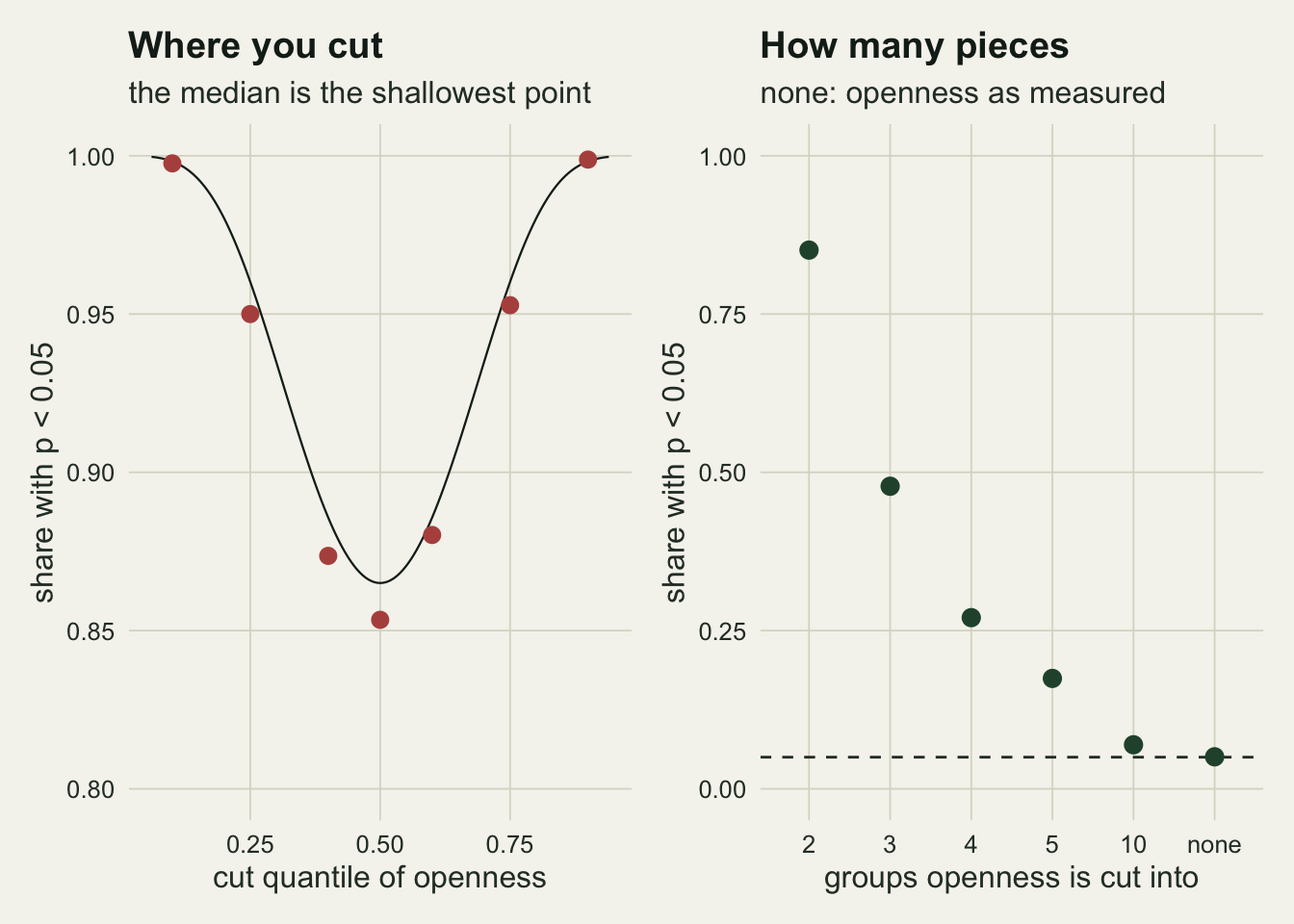
Two practical questions follow. Ecologists rarely cut at the median by choice; the cut is usually placed at a threshold with a story attached, a canopy openness of a quarter, a condition index that separates poor animals from the rest. The closed form for a cut at quantile `q` is `k(q) = 1 - phi(z_q)^2 / (q * (1 - q))`, and it is minimised at the median, so the arbitrary-looking cut is the least damaging one available.
```{r cutsweep}
q_grid <- c(0.1, 0.25, 0.4, 0.5, 0.6, 0.75, 0.9)
cut_sweep <- do.call(rbind, lapply(seq_along(q_grid), function(i)
  sim_cell(5000, n_plot, rho_base, b_open, sde_base, "split", q = q_grid[i],
           seed = 700 + i)))
cut_sweep$k <- leak_q(q_grid)
closed_gap <- max(abs(c(cut_sweep$rej - rej_closed(n_plot, rho_base, b_open, sde_base, cut_sweep$k),
                        sweep_split$rej - rej_closed(n_plot, rho_grid, b_open, sde_base, k_median))))

q_best <- q_grid[which.min(cut_sweep$rej)]
k_ratio <- leak_q(0.1) / leak_q(0.5)
rej_gap <- max(cut_sweep$rej) - min(cut_sweep$rej)
round(cut_sweep[, c("q", "k", "rej", "se_rej", "bias")], 4)
```
Cutting at the tenth percentile leaves `r sprintf("%.4f", cut_sweep$k[1])` of the openness axis unadjusted, `r sprintf("%.2f", k_ratio)` times what the median cut leaves, and the false-positive rate there is `r sprintf("%.4f", cut_sweep$rej[1])`. The sweep is symmetric about `r sprintf("%.1f", q_best)`, which is where it bottoms out, and the spread between the best and the worst cut is `r sprintf("%.3f", rej_gap)`. A threshold chosen for biological meaning, away from the middle of the distribution, is worse than the median split it was meant to improve on, and it is worse for a reason that has nothing to do with biology: the two groups are more unequal in size, so the indicator carries less of the variable. The other question is grain. Tertiles, quartiles and deciles are all coarsenings, and the leak falls quickly as the pieces get smaller.
```{r grain}
grain_adj <- c("split", "3", "4", "5", "10", "cont")
grain <- do.call(rbind, lapply(seq_along(grain_adj), function(i)
  sim_cell(5000, n_plot, rho_base, b_open, sde_base, grain_adj[i], seed = 810 + i)))

leak_cuts <- function(cuts) {
  dz <- c(0, dnorm(qnorm(cuts)), 0)
  1 - sum(diff(dz)^2 / diff(c(0, cuts, 1)))
}
grain$k <- c(leak_q(0.5), leak_cuts(1:2 / 3), leak_cuts(1:3 / 4),
             leak_cuts(1:4 / 5), leak_cuts(1:9 / 10), 0)
grain$groups <- factor(c("2", "3", "4", "5", "10", "none"),
                       levels = c("2", "3", "4", "5", "10", "none"))
dec_z <- (grain$rej[5] - 0.05) / grain$se_rej[5]
round(setNames(grain$rej, grain$groups), 4)
```
Tertiles bring the rate to `r sprintf("%.4f", grain$rej[2])`, quartiles to `r sprintf("%.4f", grain$rej[3])` with the leak down to `r sprintf("%.4f", grain$k[3])`, and quintiles to `r sprintf("%.4f", grain$rej[4])`. Deciles get to `r sprintf("%.4f", grain$rej[5])`, with a bias of `r sprintf("%.4f", grain$bias[5])` that is small but not zero, and the rate is still `r sprintf("%.1f", dec_z)` Monte Carlo standard errors above nominal. Leaving openness as measured returns `r sprintf("%.4f", grain$rej[6])`. Fine grain is not the same as no grain, and the only cell in the table that is actually at the advertised level is the one with no cutting in it. One bookkeeping note before the figure: the median cell appears in all three sweeps above, with a different seed each time, and it comes out at `r sprintf("%.4f", rej_split_base)`, `r sprintf("%.4f", cut_sweep$rej[4])` and `r sprintf("%.4f", grain$rej[1])`. The spread is Monte Carlo noise, and the first of the three is the one quoted as the headline.
```{r figcut}
#| fig-cap: "Where the cut is placed, and how many pieces it makes. Left: the closed-form rate as a curve running a little above the simulated cuts through the middle of the range. Right: rates for two to ten equal groups against the uncut covariate."
#| fig-alt: "Two panels on warm off-white paper. The left panel plots the share of significant surveys against the quantile used as the cut, on a vertical axis running from eight tenths to one, with red dots at seven cut points and a dark curve that runs a little above them near the centre, forming a U whose minimum is at the median and whose arms climb to almost one hundred per cent at the tenth and ninetieth percentiles. The right panel plots green dots against the number of groups, falling steeply from about eighty five per cent at two groups through forty eight and twenty seven per cent at three and four groups to seven per cent at ten groups, and the last point, labelled none, sitting on the dashed five per cent line."
cut_curve <- data.frame(q = seq(0.06, 0.94, length.out = 200))
cut_curve$rej <- rej_closed(n_plot, rho_base, b_open, sde_base, leak_q(cut_curve$q))

p_cut <- ggplot(cut_sweep, aes(q, rej)) +
  geom_line(data = cut_curve, aes(q, rej), colour = te_ink, linewidth = 0.4) +
  geom_point(size = 2.6, colour = te_rust) +
  scale_y_continuous(limits = c(0.8, 1)) +
  labs(x = "cut quantile of openness", y = "share with p < 0.05",
       title = "Where you cut", subtitle = "the median is the shallowest point") +
  theme_datasheet()

p_grain <- ggplot(grain, aes(groups, rej)) +
  geom_hline(yintercept = 0.05, linetype = "dashed", colour = te_body, linewidth = 0.5) +
  geom_point(size = 2.8, colour = te_forest) +
  scale_y_continuous(limits = c(0, 1)) +
  labs(x = "groups openness is cut into", y = "share with p < 0.05",
       title = "How many pieces", subtitle = "none: openness as measured") +
  theme_datasheet()

p_cut + p_grain + plot_annotation(theme = theme_datasheet())
```
## What to report
Put the covariate in the model on the scale it was measured on. The two-class version can still appear in the figures and in the abstract, where it is a description and costs nothing; the harm starts when the classes replace the numbers in the model that produces the p value.
If a covariate has to be presented in groups, say which quantiles the cuts sit at and how they were chosen, and give the number of plots in each group. A cut at a fifth or a tenth of the distribution is not equivalent to a median cut, and a reader cannot tell what was done from the phrase high versus low. If groups are unavoidable, more of them are better: quartiles remove most of the distortion and deciles nearly all of it, at the price of parameters the survey has to pay for. Royston, Altman and Sauerbrei (2006) make the general recommendation, and a spline is usually the better answer if the reason for cutting was a suspected nonlinear response.
State the correlation between the grouped covariate and the predictor of interest. That correlation enters the bias multiplied by the covariate's effect on the response, so neither quantity settles the question on its own. At a fixed correlation the bias grows in proportion to that effect, so a correlation small enough to ignore in one survey is not small enough in another where the covariate has a firmer hold on the response. The sweep above moves the correlation with that effect held at `r sprintf("%g", b_open)`, and even at that setting the split sits above the advertised level at every non-zero correlation on the grid.
Report the direction as well as the size. The spurious coefficient takes the sign of the product of the covariate's effect and the covariate to predictor correlation, so it lands wherever those two point, which is often the direction the study expected. A result that agrees with the hypothesis is not evidence that the adjustment worked.
## Honest limits
The asymptotics here are closed form, and the simulations confirm them rather than discover them. The leak, the bias and the noncentral t rejection rate are all algebra for a normal covariate under a two-sided t test, and across the seven cut points and the thirteen correlations the prediction and the simulation differ by at most `r sprintf("%.4f", closed_gap)`, the prediction sitting above the simulation wherever that gap is widest. The likely source of that gap is the finite-sample cost of estimating the cut from the data rather than knowing it, but nothing here isolates it. What the simulation genuinely adds is the finite-sample behaviour of the estimated cut point. Reading the headline rate as a constant of nature is the mistake this structure is meant to prevent.
The `k = 1 - 2/pi` figure quoted throughout is the normal case, which is the mild one. Right-skewed covariates are the rule in field ecology, and a lognormal covariate leaves roughly twice as much behind. A survey that cuts a strongly skewed variable at its median is further from the numbers in this post than the numbers suggest, and in the wrong direction.
The reassurance that a linear term is enough assumes the dependence between covariate and predictor is linear, which is what joint normality delivers. One nonlinear-dependence design was tried above and the linear adjustment held its level, but a single cell is not a general result, and a covariate whose association with the exposure is genuinely curved needs a spline on the covariate rather than a straight line. Everything here uses one confounder, a Gaussian response, no interactions and a correctly specified exposure variable. Two correlated confounders, one grouped and one not, is the obvious next case and it is untested here. Nothing in this post speaks to splitting the predictor of interest rather than the confounder either, which is a power question with a different answer: Cohen (1983) worked out the cost, and MacCallum and colleagues (2002) collected the cases where the practice manufactures effects rather than merely losing them.
## References
Austin PC, Brunner LJ 2004 Statistics in Medicine 23(7):1159-1178 (10.1002/sim.1687)
Becher H 1992 Statistics in Medicine 11(13):1747-1758 (10.1002/sim.4780111308)
Cohen J 1983 Applied Psychological Measurement 7(3):249-253 (10.1177/014662168300700301)
MacCallum RC, Zhang S, Preacher KJ, Rucker DD 2002 Psychological Methods 7(1):19-40 (10.1037/1082-989X.7.1.19)
Royston P, Altman DG, Sauerbrei W 2006 Statistics in Medicine 25(1):127-141 (10.1002/sim.2331)
## Related tutorials
- [Measurement error and regression dilution](../measurement-error-regression-dilution/)
- [Baseline selection and the return to the mean](../baseline-selection-and-the-return-to-mean/)
- [Confounding and backdoor adjustment](../confounding-and-backdoor-adjustment/)
- [Sensitivity to unmeasured confounding](../sensitivity-to-unmeasured-confounding/)