Ordinal regression for ordered cover classes

Braun-Blanquet cover classes are ordered categories, not numbers. Fit a proportional-odds model from scratch in R, check the parallel-slopes assumption, and read the odds ratio.

Vegetation surveys rarely record cover as a precise percentage. They record a class: the Braun-Blanquet scale, or something like it, sorting each quadrat into a handful of ordered bins such as less than 5 percent, 5 to 25, 25 to 50, and so on. The classes have a clear order but no meaningful spacing. The jump from class 1 to class 2 is not the same amount of cover as the jump from class 4 to class 5, and there is no such thing as class 3.7.

The reflex is to type the classes as the numbers 1 to 5 and run ordinary regression. That treats an order as if it were a measurement, and it answers a question you did not ask. This post fits the model built for ordered categories, the proportional-odds cumulative logit, by hand, cross-checks it against MASS::polr, and shows how to test the one assumption it rests on.

The proportional-odds model

The idea is to model the cumulative probability of being at or below each class. With classes ordered from 1 to J and a covariate x, the model is logit P(Y <= j) = theta_j - x beta, where the cutpoints theta_1 < theta_2 < ... < theta_{J-1} set the baseline splits and a single slope beta shifts every split together. That shared slope is the proportional-odds assumption: a unit of x multiplies the odds of being in a higher class by the same factor at every threshold. The pay-off is one interpretable number, an odds ratio, instead of a separate model per split.

We simulate cover classes along a soil-moisture gradient with a genuine slope of 1.25 and four unequally spaced cutpoints.

set.seed(4227)
n    <- 260
x    <- round(runif(n, -2, 2), 3)
beta <- 1.25
th   <- c(-1.6, -0.4, 0.9, 2.1)                       # four cutpoints, unequal spacing
Pcum <- cbind(sapply(th, function(t) plogis(t - beta * x)), 1)
Pcat <- cbind(Pcum[, 1], t(apply(Pcum, 1, diff)))     # per-class probabilities
y    <- apply(Pcat, 1, function(p) sample(1:5, 1, prob = p))

Fitting proportional odds from scratch

We maximise the multinomial log-likelihood of the observed classes. The only trick is keeping the cutpoints ordered: parameterise the first cutpoint freely and the gaps as exponentials, so theta is always increasing.

negll_po <- function(par, y, x) {
  b   <- par[1]
  th  <- cumsum(c(par[2], exp(par[3:5])))             # ordered cutpoints
  Pc  <- plogis(outer(th, b * x, "-"))                # (J-1) x n cumulative
  Pc  <- rbind(Pc, 1)
  Pk  <- rbind(Pc[1, ], apply(Pc, 2, diff))           # J x n category probs
  -sum(log(pmax(Pk[cbind(y, seq_along(y))], 1e-12)))
}
fit <- optim(c(0, -1.5, log(1.2), log(1.3), log(1.2)),
             negll_po, y = y, x = x, method = "BFGS", hessian = TRUE)
bh  <- fit$par[1]
thh <- cumsum(c(fit$par[2], exp(fit$par[3:5])))
p227_b  <- round(bh, 3)
p227_bse <- round(sqrt(diag(solve(fit$hessian)))[1], 3)
p227_or <- round(exp(bh), 2)

The estimated slope is 1.313 (SE 0.128) on the log-odds scale, which recovers the truth of 1.25. Exponentiating gives an odds ratio of 3.72: each unit of soil moisture multiplies the odds of falling in a higher cover class by that factor, and by the proportional-odds assumption this holds at every threshold.

Cross-checking against MASS::polr

The from-scratch fit should match the standard implementation exactly, since both maximise the same likelihood.

suppressWarnings(suppressMessages(library(MASS)))
pol <- polr(factor(y, ordered = TRUE) ~ x, method = "logistic", Hess = TRUE)
p227_dbeta <- signif(abs(bh - coef(pol)), 2)
p227_dcut  <- signif(max(abs(thh - pol$zeta)), 2)

The hand-coded slope matches polr to 6^{-7} and the cutpoints agree to 3.3^{-5}, so the implementation is correct. From here we could use either; the point of the by-hand version is that nothing about the model is hidden.

Reading category probabilities

Because the model is built from cumulative probabilities, it returns the full probability of every class at any covariate value. This is what an ecologist actually wants: not a single number, but how the class composition changes along the gradient.

Figure 1: Predicted probability of each cover class along the soil-moisture gradient from the proportional-odds model. As moisture rises, probability mass moves smoothly from the low classes to the high classes.

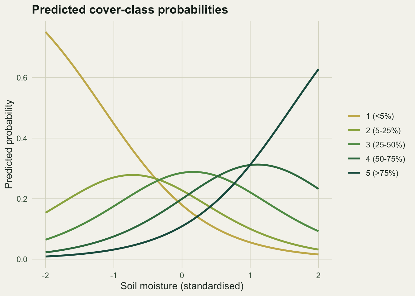
Why the numeric-code shortcut is the wrong tool

Fit ordinary regression on the class codes and the trouble is not a subtle bias; it is that the output means nothing.

ols <- lm(y ~ x)
p227_pred <- round(predict(ols, data.frame(x = 2)), 2)
p227_sp   <- round(cor(x, y, method = "spearman"), 3)

At high moisture the linear model predicts a class of 4.49. There is no class 4.49; the categories are labels, not quantities. The model also cannot tell you the probability of any class, which is the quantity of interest. And it forces the assumption the cover scale explicitly denies: that the classes are equally spaced, so that class 1 to 2 counts the same as class 4 to 5. The proportional-odds model uses only the order (its rank correlation with moisture is 0.618, in the same direction), assigns no scores, and returns probabilities and an odds ratio instead of a phantom fractional class.

Testing the parallel-slopes assumption

Proportional odds buys interpretability by assuming one slope fits every threshold. That assumption can fail: an environmental driver might matter far more for crossing from sparse to moderate cover than from moderate to dense. The simplest visual check fits a separate binary logistic regression at each split, comparing “above class j” to “at or below j”, and asks whether the slopes agree.

sep_slopes <- function(y, x) sapply(1:4, function(j) coef(glm((y > j) ~ x, family = binomial))[2])
ss_po <- sep_slopes(y, x)
p227_spreadPO <- round(diff(range(ss_po)), 3)

set.seed(4228)                                         # a non-proportional counterexample
x2 <- round(runif(n, -2, 2), 3)
bj <- c(0.4, 0.9, 1.6, 2.4)                            # effect grows across thresholds
Pc2 <- cbind(sapply(1:4, function(j) plogis(th[j] - bj[j] * x2)), 1)
Pk2 <- cbind(Pc2[, 1], t(apply(Pc2, 1, diff))); Pk2 <- pmax(Pk2, 0); Pk2 <- Pk2 / rowSums(Pk2)
y2  <- apply(Pk2, 1, function(p) sample(1:5, 1, prob = p))
ss_np <- sep_slopes(y2, x2)
p227_spreadNP <- round(diff(range(ss_np)), 3)

For proportional-odds data the four threshold slopes cluster tightly (spread 0.218), close to the common value the model estimates. For the non-proportional counterexample they fan from about 0.63 to 2.06 (spread 1.427): a single slope cannot describe them, and forcing one would misstate the effect at both ends.

Figure 2: Slopes from separate binary logistic regressions at each class threshold. When proportional odds holds the slopes cluster near a common value (dashed line); when it fails they fan out, and a single-slope model no longer fits.

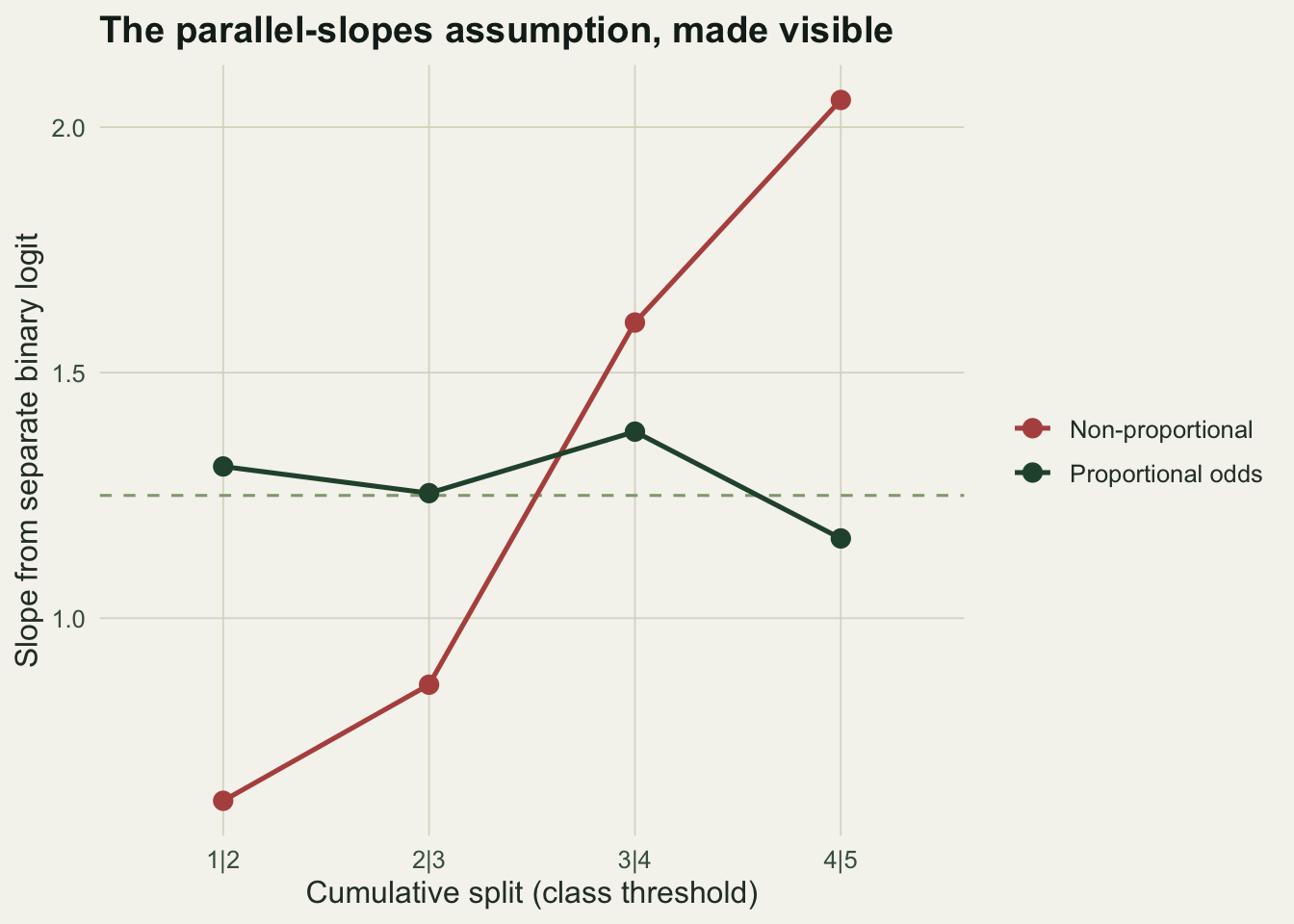
The formal version of this eyeball test is Brant’s test, which compares the threshold-specific slopes against a common slope with a chi-square statistic. The companion post on checking a bounded-response model runs it and adds residual diagnostics.

Where this leaves us

Ordered categories deserve a model that uses the order and nothing more. Proportional odds does exactly that: it gives the probability of every class along the gradient and a single odds ratio for the effect, without pretending the classes are equally spaced numbers or inventing fractional categories. It asks one thing in return, that a single slope fits every threshold, and that is checkable. When the parallel-slopes plot fans out, the honest response is a partial-proportional-odds model that frees the offending slope, or a different ordinal link. When it holds, one odds ratio tells the whole story.

Related tutorials

• Beta regression for proportion and cover data
• Tweedie regression for biomass and cover with zeros
• Checking a bounded-response model
• Logistic regression for presence-absence data

References

McCullagh P 1980 Journal of the Royal Statistical Society Series B 42(2):109-142 (10.1111/j.2517-6161.1980.tb01109.x)

Brant R 1990 Biometrics 46(4):1171-1178 (10.2307/2532457)

Guisan A, Harrell FE 2000 Journal of Vegetation Science 11(5):617-626 (10.2307/3236568)

Venables WN, Ripley BD 2002 Modern Applied Statistics with S, fourth edition, ISBN 978-0-387-95457-8