set.seed(4284)
n   <- 180
x   <- round(runif(n, -2, 2), 3)          # standardised soil moisture
b0  <- 0.4; b1 <- 1.15                     # true mean model (logit scale)
phi <- 9                                   # true precision
mu  <- plogis(b0 + b1 * x)
y <- rbeta(n, mu * phi, (1 - mu) * phi) # cover as a proportion in (0, 1)Beta regression for proportion and cover data
R
ecology tutorial
regression
GLM
proportions
Vegetation cover and other continuous proportions live between zero and one. Fit beta regression from scratch in R, and see why logit plus OLS is biased.
Per cent cover, the fraction of seeds that germinate, the share of foraging time spent vigilant: continuous proportions turn up across ecology, and they share an awkward feature. They are bounded in the open interval between zero and one, and their variance is not constant. A proportion near 0.5 can vary a lot; one near 0 or 1 is pinned by the boundary and can vary only a little. Ordinary linear regression ignores both facts. It will happily predict a cover of 1.3 or minus 0.2, and it assumes the scatter is the same everywhere.
The usual patch is a transform: take the logit or the arcsine square root of the proportion and run OLS on that. This post shows why that patch is biased for genuinely continuous proportions, and fits the honest alternative, beta regression, by hand. The response is assumed to follow a beta distribution whose mean is modelled on the logit scale, exactly the shape the data have.
The beta distribution, parameterised for regression
The beta distribution has two shape parameters, but for regression it is far more useful to reparameterise it by a mean and a precision. Write the mean as mu and the precision as phi; then the two shapes are mu * phi and (1 - mu) * phi, and the variance is mu (1 - mu) / (phi + 1). Larger phi means tighter scatter. The mean depends on covariates through a logit link, logit(mu) = X beta, so the coefficients read like a logistic regression: a slope is a change in log-odds of the expected proportion.
We simulate vegetation cover along a soil-moisture gradient, with a genuine mean-slope of 1.15 on the logit scale and a constant precision of 9.
Fitting beta regression from scratch
There is no closed-form estimator, so we maximise the beta log-likelihood directly. The mean is plogis(X beta), the precision is exp(gamma) to keep it positive, and dbeta gives the density on the reparameterised shapes.
negll <- function(par, y, X) {
  k   <- ncol(X)
  mu  <- plogis(X %*% par[1:k])
  phi <- exp(par[k + 1])
  -sum(dbeta(y, mu * phi, (1 - mu) * phi, log = TRUE))
}
X   <- cbind(1, x)
fit <- optim(c(0, 0, log(5)), negll, y = y, X = X, method = "BFGS", hessian = TRUE)
stopifnot(fit$convergence == 0)   # check before inverting the Hessian
bh  <- fit$par[1:2]
phih <- exp(fit$par[3])
se  <- sqrt(diag(solve(fit$hessian)))     # asymptotic SE from the Hessian
p226_b1  <- round(bh[2], 3)
p226_b1se <- round(se[2], 3)
p226_phi <- round(phih, 2)
The estimated mean-slope is 1.154 (SE 0.053) and the precision is 9, recovering the true values of 1.15 and 9. A quick sanity check confirms we are at a genuine optimum: the numerical score is essentially zero at the solution.
g <- sapply(1:3, function(j) {
  e <- 1e-6; p1 <- fit$par; p2 <- fit$par; p1[j] <- p1[j] - e; p2[j] <- p2[j] + e
  (negll(p2, y, X) - negll(p1, y, X)) / (2 * e)
})
p226_score <- signif(max(abs(g)), 2)
The largest score component is \(1.3 \times 10^{-4}\), so the fit has converged.
Why the transform-and-OLS patch is biased
The tempting shortcut is to logit-transform the proportion and run OLS. It looks reasonable, but it estimates the wrong quantity. The mean of the logit is not the logit of the mean (Jensen’s inequality), so the transformed regression does not target the mean-slope we care about.
ols <- lm(qlogis(y) ~ x)
p226_ols <- round(coef(ols)[2], 3)
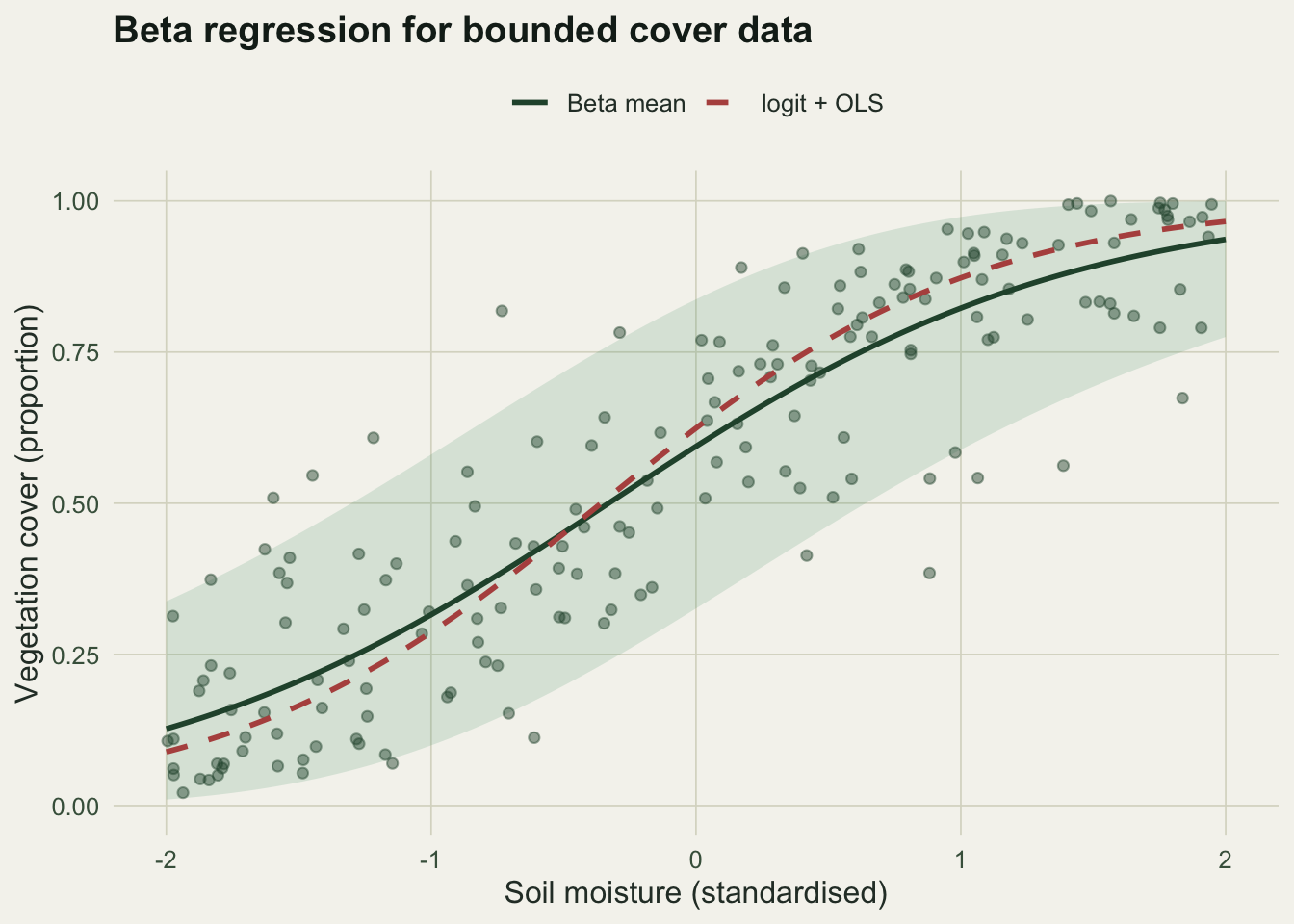
The logit-plus-OLS slope here is 1.418, well above the true 1.15. The figure below shows the fitted beta mean with its prediction band next to the OLS fit. Note that the beta prediction interval is asymmetric and stays inside zero and one, narrowing towards the boundaries exactly as the data do.
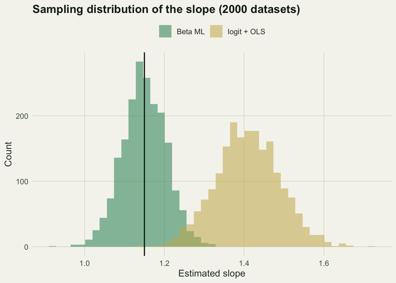
One realisation is anecdote. To see that the bias is systematic, we resample 2000 datasets from the same truth and compare the slope from each method.
set.seed(101)
B <- 2000
sb <- so <- numeric(B)
for (b in 1:B) {
  mb <- plogis(b0 + b1 * x)
  yb <- rbeta(n, mb * phi, (1 - mb) * phi)
  sb[b] <- optim(c(0, 0, log(5)), negll, y = yb, X = X, method = "BFGS")$par[2]
  so[b] <- coef(lm(qlogis(yb) ~ x))[2]
}
p226_biasBeta <- round(100 * (mean(sb) - b1) / b1, 1)
p226_biasOls  <- round(100 * (mean(so) - b1) / b1, 1)
p226_sdratio  <- round(sd(so) / sd(sb), 2)
Across the 2000 datasets the beta estimator is unbiased (0% relative bias), while logit-plus-OLS is biased upward by 22.5%. Beta is also more precise: the OLS slope has 1.46 times the standard deviation of the beta slope. The transform costs both accuracy and efficiency.
Modelling the precision: variable dispersion
A strength of beta regression that no transform offers is a submodel for the precision. Ecological scatter is rarely constant; it often tightens or loosens along a gradient. We let log(phi) depend on the same covariate, so the model has a mean part and a dispersion part, and compare it to a constant-precision fit with a likelihood-ratio test.
set.seed(4285)
xd  <- round(runif(n, -2, 2), 3)
mud <- plogis(0.3 + 0.9 * xd)
phid <- exp(2.4 - 0.7 * xd)                 # precision shrinks as moisture rises
yd  <- rbeta(n, mud * phid, (1 - mud) * phid)
Xd  <- cbind(1, xd)
nll_c <- function(p) { mu <- plogis(Xd %*% p[1:2]); ph <- exp(p[3])
  -sum(dbeta(yd, mu * ph, (1 - mu) * ph, log = TRUE)) }
nll_v <- function(p) { mu <- plogis(Xd %*% p[1:2]); ph <- exp(Xd %*% p[3:4])
  -sum(dbeta(yd, mu * ph, (1 - mu) * ph, log = TRUE)) }
fc <- optim(c(0, 0, log(5)), nll_c, method = "BFGS")
fv <- optim(c(0, 0, 2, 0), nll_v, method = "BFGS")
LR <- 2 * (fc$value - fv$value)
p226_g1   <- round(fv$par[4], 3)
p226_LR   <- round(LR, 1)
p226_LRp  <- signif(pchisq(LR, 1, lower.tail = FALSE), 3)
p226_dAIC <- round(2 * (fc$value - fv$value) - 2, 1)
The dispersion-slope is estimated at -0.811 (the truth is minus 0.7), and the variable-precision model is a decisive improvement (likelihood-ratio 72.1, p equal to \(2.03 \times 10^{-17}\), delta-AIC 70.1). A constant-variance model would have missed this structure entirely, and would have reported misleading intervals in the region where the scatter is actually widest.
The boundary: exact zeros and ones
Field proportions often include exact zeros (bare ground) and exact ones (complete cover). The beta density is not defined at zero or one, so the log-likelihood is negative infinity if any observation sits on the boundary. The standard fix, from Smithson and Verkuilen, is a small squeeze that pulls the endpoints just inside: replace each y by (y (n - 1) + 0.5) / n.
set.seed(4286)
xb2  <- round(runif(120, -2, 2), 3)
mub2 <- plogis(0.2 + 0.8 * xb2)
yb2  <- rbeta(120, mub2 * 7, (1 - mub2) * 7)      # precision fixed at 7 across the gradient
yb2[sample(120, 6)] <- 0
yb2[sample(120, 4)] <- 1
n2  <- length(yb2)
ysv <- (yb2 * (n2 - 1) + 0.5) / n2
p226_nzero <- sum(yb2 == 0)
p226_none  <- sum(yb2 == 1)
p226_sv0   <- round(min(ysv), 4)
Here 6 observations are exactly zero and 4 are exactly one. The squeeze maps the zeros to 0.0042, a value the beta density can handle, and leaves the interior points barely touched. This is a pragmatic device, not a free lunch: if a large share of the data sits on the boundary, the response is really a mixture of a point mass and a continuous part, and a zero-and-one-inflated model is the honest description.
The honest boundary: continuous proportion or count proportion?
Beta regression is for proportions that are genuinely continuous, where there is no underlying count. That distinction matters. If your proportion is instead the number of successes out of a known number of trials (12 of 20 seeds germinated), the data are binomial, and logistic regression is both correct and more efficient, because it uses the trial count: a proportion from few trials is noisier than one from many, and a binomial model knows this while a constant-precision beta model does not.
set.seed(4287)
ntr <- round(runif(150, 8, 25))
xc  <- round(runif(150, -2, 2), 3)
pc  <- plogis(0.3 + 1.0 * xc)
k   <- rbinom(150, ntr, pc)
bin <- glm(cbind(k, ntr - k) ~ xc, family = binomial)
p226_bin   <- round(coef(bin)[2], 3)
p226_binse <- round(summary(bin)$coefficients[2, 2], 3)
For these count-based proportions the binomial slope is 1.04 (SE 0.046), recovering the truth of 1.0 while giving each observation the weight its sample size deserves. The rule of thumb is simple: successes out of a total go to logistic regression; a genuinely continuous fraction with no denominator goes to beta regression. As Warton and Hui put it, reaching for the arcsine transform in either case is the wrong move.
Where this leaves us
Beta regression fits proportions on the scale they actually occupy, gives interpretable log-odds coefficients, models the changing scatter through a precision submodel, and produces prediction intervals that respect the boundaries. The transform-and-OLS habit does none of these and pays for it in bias and lost power. The one judgement it still asks of you is whether the response is a continuous fraction or a count proportion, and whether the boundary mass is small enough to squeeze or large enough to model. The companion post on checking a bounded-response model returns to that judgement with residual diagnostics.
References
Ferrari S, Cribari-Neto F 2004 Journal of Applied Statistics 31(7):799-815 (10.1080/0266476042000214501)
Smithson M, Verkuilen J 2006 Psychological Methods 11(1):54-71 (10.1037/1082-989X.11.1.54)
Warton DI, Hui FKC 2011 Ecology 92(1):3-10 (10.1890/10-0340.1)
Douma JC, Weedon JT 2019 Methods in Ecology and Evolution 10(9):1412-1430 (10.1111/2041-210X.13234)