set.seed(4230)
n   <- 400
x   <- round(runif(n, -2, 2), 3)               # standardised environmental gradient
b0  <- -0.3; b1 <- 0.9                          # true log-mean model
p   <- 1.55                                     # true Tweedie power in (1, 2)
phi <- 1.4                                      # true dispersion
mu  <- exp(b0 + b1 * x)
lam <- mu^(2 - p) / (phi * (2 - p))             # Poisson rate of clumps
shp <- (2 - p) / (p - 1)                        # gamma shape per clump
scl <- phi * (p - 1) * mu^(p - 1)               # gamma scale
N   <- rpois(n, lam)
y   <- vapply(seq_len(n), function(i)
         if (N[i] == 0) 0 else sum(rgamma(N[i], shape = shp, scale = scl[i])), numeric(1))
p228_zf   <- round(mean(y == 0), 3)
p228_mean <- round(mean(y), 2)
p228_p0 <- round(mean(exp(-lam)), 3)Tweedie regression for biomass and cover with zeros
R
ecology tutorial
regression
GLM
Biomass and catch per unit effort mix exact zeros with a skewed positive part. Fit Tweedie regression with mgcv, and see why logging with a constant is biased.
Corrected 7 October 2026: the profile of the Tweedie power plugged in the dispersion from each fit instead of maximising over it, which made the curve too steep in the tails and put its peak one grid step low; the code now maximises over the dispersion, and the text, caption and alt text describe the corrected curve. The post also said that the companion post on model checking returns to the one-process-or-two question with residual diagnostics for both models; it now says that post comes back to it only briefly.
Aboveground biomass, catch per unit effort, per cent cover measured on a continuous scale: these responses share a shape that trips up the standard toolbox. They are non-negative, they carry a spike of exact zeros where the species was absent or nothing was caught, and their positive part is continuous and right-skewed. A Gaussian model ignores the zeros and the skew. A gamma or lognormal model has no room for a zero at all, since both live on the strictly positive numbers: an exact zero carries probability zero and the likelihood is undefined there. The usual escape, adding a small constant and taking logs, quietly changes the answer depending on the constant you pick.
This post fits the distribution built for exactly this situation, the Tweedie, using mgcv. The Tweedie with a power parameter between one and two is the compound Poisson-gamma: a point mass at zero glued to a skewed continuous density above it, in a single likelihood with a single mean model. We simulate it from scratch so the mechanism is visible, recover the mean-slope and the power, and compare it with the log-plus-constant habit and with a two-part model.
The Tweedie family and its power parameter
Tweedie distributions are the exponential-dispersion family whose variance is a power of the mean, Var(Y) = phi * mu^p. The power p selects the shape: p = 1 is Poisson-like, p = 2 is the gamma, and any p strictly between one and two is a compound Poisson-gamma, a random number of gamma-distributed clumps. That intermediate case is the ecological one, because it is the only member of the family that places positive probability on an exact zero while keeping the positive part continuous. The probability of a zero is exp(-mu^(2 - p) / (phi (2 - p))), so the same mean that drives the positive values also sets how often you see a zero.
We simulate biomass along an environmental gradient as an explicit compound Poisson-gamma: draw a Poisson count of clumps, then sum that many gamma variables. A count of zero clumps gives an exact zero.
A share of 0.238 of the values are exact zeros, the mean biomass is 1.24, and the closed-form zero probability averaged over the gradient is 0.27, a little above the simulated share: the closed form gives the expected fraction, and a single simulated sample scatters around it. The zeros are not missing data or rounding; they are a genuine part of the distribution.
Fitting Tweedie with mgcv
mgcv fits Tweedie regression and, with the tw() family, estimates the power parameter by restricted maximum likelihood alongside the mean model. The mean is on a log link, so its coefficients read like a Poisson or gamma GLM.
suppressWarnings(suppressMessages(library(mgcv)))
f_tw <- gam(y ~ x, family = tw(), method = "REML")
p228_slope <- round(coef(f_tw)[2], 3)
p228_se    <- round(summary(f_tw)$p.table[2, 2], 3)
p228_phat  <- round(f_tw$family$getTheta(TRUE), 2)
p228_phi   <- round(f_tw$scale, 2)
The estimated mean-slope is 0.943 (SE 0.054), recovering the true 0.9 while every zero contributes to the fit. The power is estimated at 1.58 and the dispersion at 1.36, close to the true 1.55 and 1.4. One model has handled the zeros and the skew together, with no transformation and no separate treatment of the absences.
pres <- as.integer(y > 0)
mb   <- glm(pres ~ x, family = binomial)                       # presence
mg   <- glm(y[pres == 1] ~ x[pres == 1], family = Gamma(link = "log"))  # positive part
xs   <- seq(-2, 2, length = 160)
m_tw <- as.vector(exp(predict(f_tw, data.frame(x = xs))))
m_dp <- plogis(coef(mb)[1] + coef(mb)[2] * xs) * exp(coef(mg)[1] + coef(mg)[2] * xs)
p228_presslope <- round(coef(mb)[2], 3)
p228_gamslope  <- round(coef(mg)[2], 3)
p228_meandiff  <- round(max(abs(m_tw - m_dp)), 3)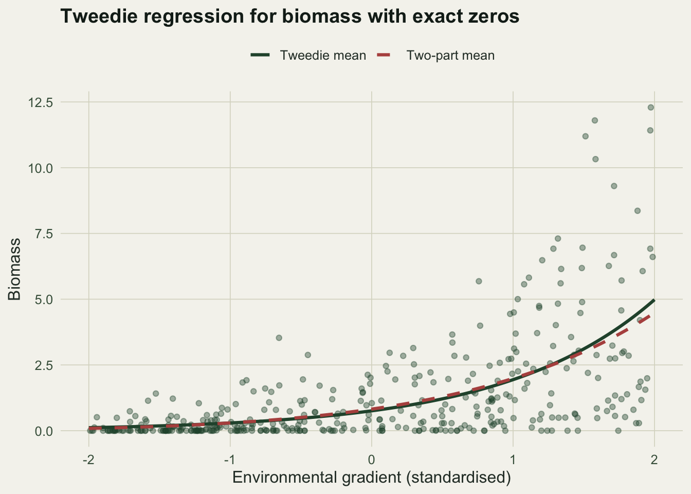
Why logging with a constant is biased
The most common shortcut is to add a small constant to clear the zeros and run OLS on log(y + c). The trouble is that c is not a nuisance you can set aside. It is a lever on the slope: different constants give different answers, and none of them target the mean on the natural scale.
cs <- c(0.1, 1, 10)
p228_logc <- round(sapply(cs, function(cc) coef(lm(log(y + cc) ~ x))[2]), 3)
With c equal to 0.1, 1 and 10 the slope comes out as 0.778, 0.347 and 0.077. The true slope is 0.9, and the estimate slides further from it as the constant grows: the constant dominates the many zeros and flattens the fitted trend. O’Hara and Kotze make the same point for counts; for semicontinuous data the fix is the same, model the response on its own scale.
The power parameter is the knob
The power p is what lets one distribution span the range from many zeros to a heavy positive tail, so it is worth estimating rather than guessing. We profile the Tweedie log-likelihood over a grid of p: for each candidate we refit the mean model and then maximise the mgcv::ldTweedie log-likelihood over the dispersion, so that every point on the curve is a profile value rather than a plug-in.
pg <- seq(1.2, 1.9, by = 0.05)
ll <- sapply(pg, function(pp) {
  fp <- gam(y ~ x, family = Tweedie(p = pp, link = "log"), method = "REML")
  # for fixed p the coefficients do not depend on the dispersion, so only phi is maximised
  -optimize(function(ph) -sum(ldTweedie(y, mu = fitted(fp), p = pp, phi = ph)[, 1]),
            c(0.05, 20))$objective
})
p228_ppeak <- pg[which.max(ll)]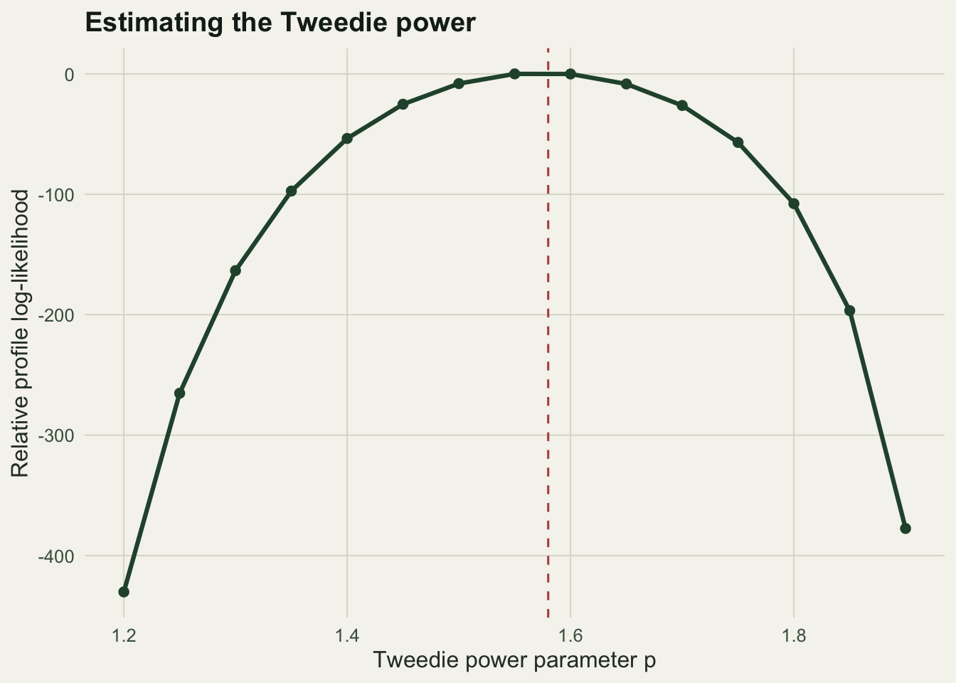
The profile peaks at 1.6, and the tw() estimate of 1.58 sits at the same place. A model that fixed p at the wrong value, or that forced p = 2 and so forbade any zero, would misdescribe the mean-variance relationship and the zero probability at once.
One realisation is anecdote
To confirm the pattern is systematic we resample 400 datasets from the same truth and compare the Tweedie slope against the log-plus-one slope.
set.seed(77)
B <- 400
st <- sp <- so <- numeric(B)
for (b in 1:B) {
  Nb <- rpois(n, lam)
  yb <- vapply(seq_len(n), function(i)
          if (Nb[i] == 0) 0 else sum(rgamma(Nb[i], shape = shp, scale = scl[i])), numeric(1))
  fb <- gam(yb ~ x, family = tw(), method = "REML")
  st[b] <- coef(fb)[2]; sp[b] <- fb$family$getTheta(TRUE)
  so[b] <- coef(lm(log(yb + 1) ~ x))[2]
}
p228_twbias <- round(100 * (mean(st) - b1) / b1, 1)
p228_pbar   <- round(mean(sp), 2)
p228_obias  <- round(100 * (mean(so) - b1) / b1, 1)
Across the 400 datasets the Tweedie slope is unbiased (0.5% relative bias) and the estimated power averages 1.55, recovering the truth. The log-plus-one slope is biased by -63.7%, far from the target. The transform is not a harmless convenience; it moves the estimate a long way.
The honest limit: one process or two?
Tweedie and the two-part model are both legitimate, and they encode a different belief about the zeros. Tweedie ties the zero probability and the positive mean together through a single mean model and the power p: absence and abundance are two faces of one process. The two-part model fits presence with one submodel and the positive amount with another, so the drivers of whether a species is there can differ from the drivers of how much. In the figure the two mean curves track each other because the data were generated by a single process, yet they still differ by up to 0.497 in places, and the two-part presence-slope (0.959) and gamma-slope (0.765) need not agree.
Which is right is an ecological question, not a statistical one. If a habitat threshold governs presence while local conditions govern biomass among the sites that clear it, the two processes are distinct and the two-part model says so. If absence is simply the low-abundance tail of one gradient, Tweedie is the more parsimonious and efficient description. The data alone will rarely settle it, so the choice should follow the biology and be stated. The companion post on checking a bounded-response model comes back to this question only briefly, to explain why no residual settles it: both models can fit the observed sample.
Where this leaves us
Tweedie regression models biomass, catch rates and continuous cover on the scale they occupy, with the zeros as part of the distribution rather than an obstacle to transform away. It recovers an interpretable log-mean slope, estimates the power that controls the balance of zeros and skew, and avoids the arbitrary constant that a log transform smuggles in. The judgement it leaves you is whether absence and abundance are one process or two, and whether the estimated power is doing real work or merely absorbing misfit, which is where diagnostics come in.
References
Jorgensen B 1987 Journal of the Royal Statistical Society Series B 49(2):127-145 (10.1111/j.2517-6161.1987.tb01685.x)
Dunn PK, Smyth GK 2005 Statistics and Computing 15(4):267-280 (10.1007/s11222-005-4070-y)
Foster SD, Bravington MV 2013 Environmental and Ecological Statistics 20(4):533-552 (10.1007/s10651-012-0233-0)
Shono H 2008 Fisheries Research 93(1-2):154-162 (10.1016/j.fishres.2008.03.006)
Wood SN, Pya N, Safken B 2016 Journal of the American Statistical Association 111(516):1548-1563 (10.1080/01621459.2016.1180986)
O’Hara RB, Kotze DJ 2010 Methods in Ecology and Evolution 1(2):118-122 (10.1111/j.2041-210X.2010.00021.x)