set.seed(4231)
n   <- 300
x   <- round(runif(n, -2, 2), 3)
mu  <- plogis(0.3 + 1.0 * x)
phi <- exp(2.3 - 0.75 * x)                       # precision shrinks as the gradient rises
y   <- rbeta(n, mu * phi, (1 - mu) * phi)
Xd  <- cbind(1, x)
nll_v <- function(p) { m <- plogis(Xd %*% p[1:2]); ph <- exp(Xd %*% p[3:4])
  -sum(dbeta(y, m * ph, (1 - m) * ph, log = TRUE)) }
nll_c <- function(p) { m <- plogis(Xd %*% p[1:2]); ph <- exp(p[3])
  -sum(dbeta(y, m * ph, (1 - m) * ph, log = TRUE)) }
fv <- optim(c(0, 0, 2, 0), nll_v, method = "BFGS")
fc <- optim(c(0, 0, 2),   nll_c, method = "BFGS")
muv <- plogis(Xd %*% fv$par[1:2]); phv <- exp(Xd %*% fv$par[3:4])
muc <- plogis(Xd %*% fc$par[1:2]); phc <- exp(fc$par[3])
rq_v <- qnorm(pbeta(y, muv * phv, (1 - muv) * phv))   # full model
rq_c <- qnorm(pbeta(y, muc * phc, (1 - muc) * phc))   # constant precision
p229_shV <- signif(shapiro.test(rq_v)$p.value, 2)
p229_shC <- signif(shapiro.test(rq_c)$p.value, 2)
p229_trV <- round(abs(cor(x, rq_v^2, method = "spearman")), 3)
p229_trC <- round(abs(cor(x, rq_c^2, method = "spearman")), 3)Checking a bounded-response model
R
ecology tutorial
regression
model checking
Deviance residuals mislead for beta, ordinal and Tweedie models. Use randomised quantile residuals, a proportional-odds test and held-out calibration instead.
Corrected 14 October 2026: the closing section said the deciding evidence always sits out of sample or in the biology, although the quantile residuals against the covariate and Brant’s test settle two of the three questions in sample; it now names a check aimed at the specific assumption as well.
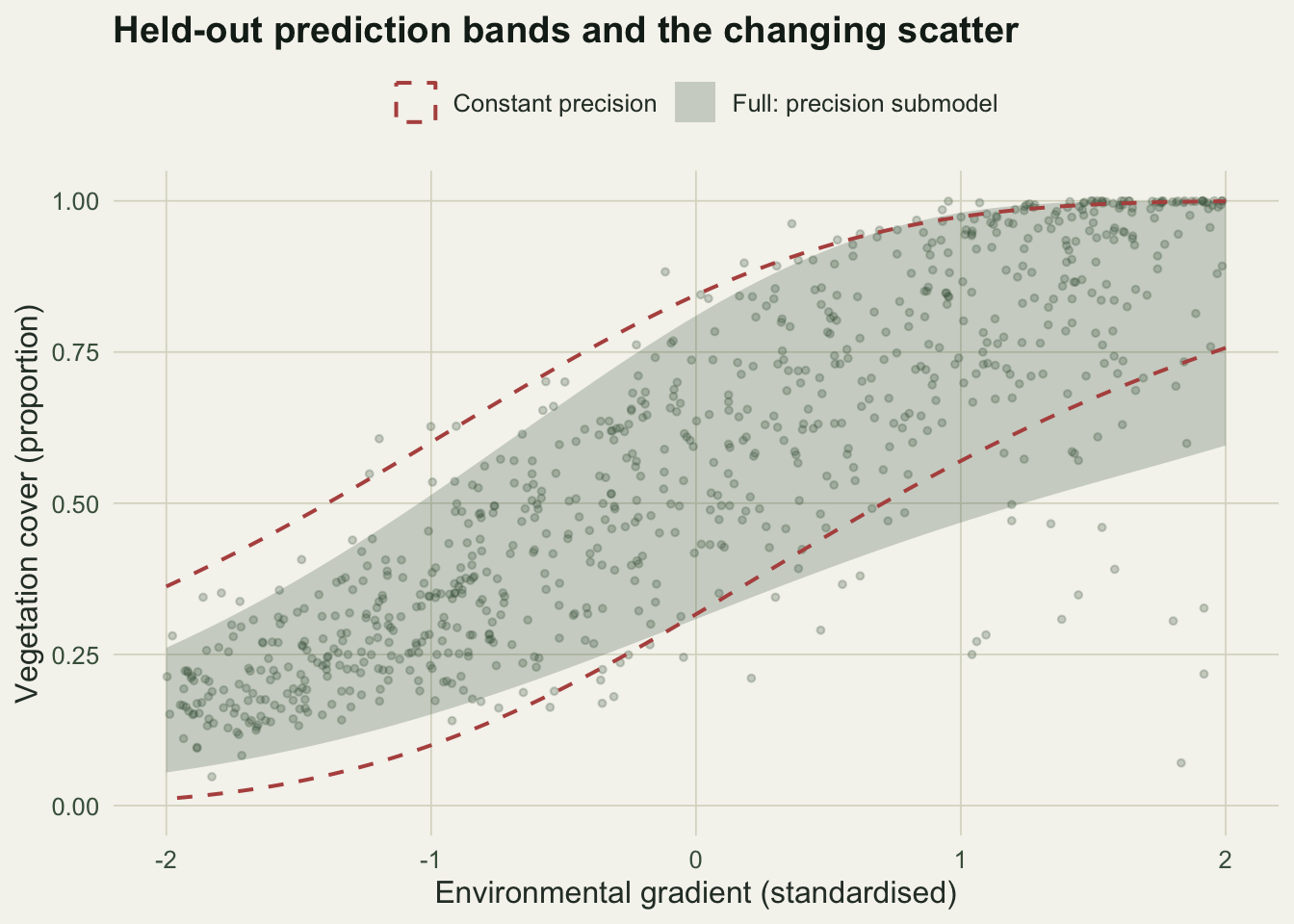
Corrected 1 October 2026: the held-out check treated the full model as the calibrated benchmark along the whole gradient; it now says that this model too covers short of nominal where the scatter is high and too much where it is low, because its estimated precision slope is shallower than the simulated one.
Corrected 27 September 2026: the caption of the held-out calibration figure said the constant-precision band keeps a fixed width; it now says the band fails to follow the changing scatter, which is what the figure shows.
The three previous posts fitted bounded and awkward responses on their own scales: beta regression for continuous proportions, proportional odds for ordered cover classes, and Tweedie for biomass with exact zeros. Each replaced a transform-and-hope habit with a model that matches the data. That raises the obvious question a fitted model always raises: how do you know it fits?
The usual residual plots do not help here. Deviance and Pearson residuals are built around a roughly Gaussian reference, and for a beta, an ordinal or a Tweedie fit they are skewed and discrete-looking even when the model is correct, so a curved residual plot tells you nothing. This post collects the checks that do work for these families: randomised quantile residuals, a formal test of the proportional-odds assumption, and out-of-sample calibration. The theme running through all three is that an in-sample summary can look clean while the model is quietly wrong, and that the honest check often lives out of sample.
Randomised quantile residuals
The residual that behaves the same way for every family is the quantile residual of Dunn and Smyth. Feed each observation through the fitted cumulative distribution function and then through the inverse normal: if the model is right, the results are standard normal whatever the response distribution, because a correctly modelled observation is a uniform draw on its own predictive distribution. For a continuous response like a proportion no randomisation is needed; for discrete parts the transform is randomised across the probability jump.
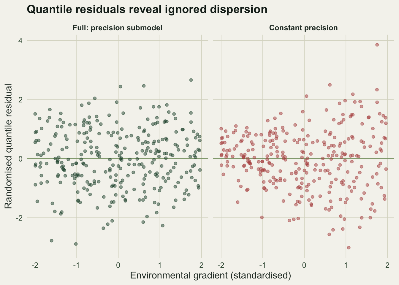
We generate cover with a precision that changes along the gradient, then fit two beta models: the full one with a precision submodel, and a constant-precision one that ignores the changing scatter.
The trap is in what a marginal test cannot see. Start with a test of overall normality. The quantile residuals of the full model give a Shapiro-Wilk p of 0.68, and the misspecified constant-precision model gives 0.41. Whichever way those two numbers fall, a marginal test of normality says nothing about where along the gradient the scatter sits. The misfit that matters here shows up when the residuals are plotted against the covariate. The squared residuals of the constant model rise with the gradient (rank correlation 0.313), the signature of scatter the model has not captured, while the full model shows no such trend (0.001).
A formal test for proportional odds
The proportional-odds post checked the parallel-slopes assumption by eye, fitting a separate binary logit at each class threshold and looking at whether the slopes clustered. Brant’s test makes that comparison formal: it asks whether the threshold-specific slopes are equal, using their joint covariance, and returns a chi-square statistic. We code it directly, which is worth doing once because it shows the test is nothing more than the eyeball plot with a covariance attached.
brant_omni <- function(y, x) {
  J <- max(y); Xb <- cbind(1, x)
  bj <- matrix(NA, J - 1, 2); pil <- matrix(NA, length(y), J - 1); Winv <- vector("list", J - 1)
  for (j in 1:(J - 1)) {
    g <- glm((y > j) ~ x, family = binomial); bj[j, ] <- coef(g)
    pj <- fitted(g); pil[, j] <- pj; Winv[[j]] <- solve(t(Xb) %*% (Xb * (pj * (1 - pj))))
  }
  P <- 2 * (J - 1); V <- matrix(0, P, P)
  for (j in 1:(J - 1)) for (l in j:(J - 1)) {                 # Brant's cross-covariance
    Vjl <- t(Xb) %*% (Xb * (pil[, max(j, l)] * (1 - pil[, min(j, l)])))
    blk <- Winv[[j]] %*% Vjl %*% Winv[[l]]
    V[(2 * j - 1):(2 * j), (2 * l - 1):(2 * l)] <- blk
    if (j != l) V[(2 * l - 1):(2 * l), (2 * j - 1):(2 * j)] <- t(blk)
  }
  si <- seq(2, P, by = 2); bs <- bj[, 2]                       # slopes only
  D <- matrix(0, J - 2, length(bs)); for (k in 1:(J - 2)) { D[k, k] <- 1; D[k, k + 1] <- -1 }
  d <- D %*% bs; Cd <- D %*% V[si, si] %*% t(D)
  stat <- as.numeric(t(d) %*% solve(Cd) %*% d)
  c(chisq = stat, df = J - 2, p = pchisq(stat, J - 2, lower.tail = FALSE))
}
set.seed(4227)                                                # proportional-odds data
nO <- 260; xO <- round(runif(nO, -2, 2), 3); th <- c(-1.6, -0.4, 0.9, 2.1)
Pc <- cbind(sapply(th, function(t) plogis(t - 1.25 * xO)), 1)
yO <- apply(cbind(Pc[, 1], t(apply(Pc, 1, diff))), 1, function(p) sample(1:5, 1, prob = p))
set.seed(4228)                                                # a non-proportional counterexample
x2 <- round(runif(nO, -2, 2), 3); bj <- c(0.4, 0.9, 1.6, 2.4)
Pc2 <- cbind(sapply(1:4, function(j) plogis(th[j] - bj[j] * x2)), 1)
Pk2 <- cbind(Pc2[, 1], t(apply(Pc2, 1, diff))); Pk2 <- pmax(Pk2, 0); Pk2 <- Pk2 / rowSums(Pk2)
y2 <- apply(Pk2, 1, function(p) sample(1:5, 1, prob = p))
bpo <- brant_omni(yO, xO); bnp <- brant_omni(y2, x2)
p229_poChi <- round(bpo["chisq"], 2); p229_poP <- round(bpo["p"], 2)
p229_npChi <- round(bnp["chisq"], 1); p229_npP <- signif(bnp["p"], 2)
For the proportional-odds data Brant’s statistic is 1.76 on 3 degrees of freedom (p equal to 0.62), no evidence against the shared slope. For the non-proportional counterexample it is 31.6 (p equal to \(6.3 \times 10^{-7}\)), decisive evidence that a single odds ratio will not do. The conclusion matches the parallel-slopes picture exactly, now with a number attached.
The honest check is out of sample
The quantile-residual trap has a larger version. A model can pass every in-sample check and still make badly calibrated predictions, because in-sample summaries reward fitting the points you have rather than the ones you do not. The cleanest test of a fitted response distribution is therefore to hold data out and ask whether its prediction intervals cover at the stated rate. We draw a large fresh sample from the same truth and check the ninety per cent intervals of both beta fits.
set.seed(909)
m  <- 4000
xt <- round(runif(m, -2, 2), 3)
yt <- rbeta(m, plogis(0.3 + xt) * exp(2.3 - 0.75 * xt), (1 - plogis(0.3 + xt)) * exp(2.3 - 0.75 * xt))
muvT <- plogis(cbind(1, xt) %*% fv$par[1:2]); phvT <- exp(cbind(1, xt) %*% fv$par[3:4])
mucT <- plogis(cbind(1, xt) %*% fc$par[1:2]); phcT <- exp(fc$par[3])
covV <- (yt >= qbeta(.05, muvT * phvT, (1 - muvT) * phvT)) & (yt <= qbeta(.95, muvT * phvT, (1 - muvT) * phvT))
covC <- (yt >= qbeta(.05, mucT * phcT, (1 - mucT) * phcT)) & (yt <= qbeta(.95, mucT * phcT, (1 - mucT) * phcT))
wide <- xt > 1; tight <- xt < -1
p229_covV <- round(mean(covV), 3);  p229_covC <- round(mean(covC), 3)
p229_wV   <- round(mean(covV[wide]), 3); p229_wC <- round(mean(covC[wide]), 3)
p229_tC   <- round(mean(covC[tight]), 3)
Overall the full model covers 0.904 of the held-out points, right on target, while the constant-precision model covers 0.885, which looks only slightly low. That overall figure hides the damage. In the high-scatter part of the gradient the constant model covers just 0.697 against the full model’s 0.846: its intervals are far too narrow exactly where the data are most variable. In the low-scatter part it covers 0.996, intervals so wide they are nearly useless. The two errors partly cancel in the average, which is why a single overall number is not enough and why the check has to be resolved along the gradient. The full model is not perfect either: its 0.846 in the high-scatter part falls short of the nominal ninety per cent, because the precision slope it estimated from 300 observations is shallower than the simulated one, and its overall figure averages that shortfall against too much coverage at low scatter. The right model removes much of the miscalibration, not all of it.
Where this leaves the series
The three families in this series each ask you to supply a piece of structure the data will not hand over on their own. Beta regression asks whether the precision is constant or varies, and the quantile residuals against a covariate are how you tell. Proportional odds asks whether one slope fits every threshold, and Brant’s test is how you tell. Tweedie asks whether absence and abundance are one process or two, a question a two-part model answers differently, and no residual settles it because both can fit the observed sample. In every case a good overall in-sample fit is necessary but not sufficient, and the deciding evidence sits in a check aimed at the specific assumption, out of sample or in the biology.
That is the same lesson the checking posts across this blog keep arriving at from different directions: an effect size needs its no-effect scale, a prediction needs a reference frame, an extrapolation needs a stated range, an interval needs its tail checked, an estimated smoothness needs its uncertainty, and a fitted distribution needs its calibration confirmed on data it has not seen. Bounded and semicontinuous responses are no exception. Fit the model the data deserve, then check it where checking is hard.
References
Dunn PK, Smyth GK 1996 Journal of Computational and Graphical Statistics 5(3):236-244 (10.1080/10618600.1996.10474708)
Brant R 1990 Biometrics 46(4):1171-1178 (10.2307/2532457)
Ferrari S, Cribari-Neto F 2004 Journal of Applied Statistics 31(7):799-815 (10.1080/0266476042000214501)
Smithson M, Verkuilen J 2006 Psychological Methods 11(1):54-71 (10.1037/1082-989X.11.1.54)
Gneiting T, Balabdaoui F, Raftery AE 2007 Journal of the Royal Statistical Society Series B 69(2):243-268 (10.1111/j.1467-9868.2007.00587.x)