---
title: "Logistic regression for presence-absence data"
description: "Model species presence and absence with a binomial GLM in R: reading log-odds and odds ratios, fitting proportion data, and spotting the separation trap."
date: "2026-06-25 11:00"
categories: [regression, GLM, species distribution, R]
image: thumbnail.png
image-alt: "A smooth logistic S-curve rising from zero to one between two horizontal guide lines."
---
A previous post worked through count data, where the response is a non-negative integer and the natural model is a Poisson or negative binomial GLM. A lot of field data is not counts but yes-or-no: a species is present or absent at a site, a seed germinates or it does not, a quadrat is occupied or empty. That binary response needs a different member of the same GLM family, the binomial model with a logit link, and it is the workhorse behind presence-absence species distribution models (Guisan and Zimmermann 2000).
This post covers the three things that trip people up: reading the coefficients on the right scale, handling proportion data without resorting to a transformation, and recognising complete separation when it wrecks a fit. Everything runs in base R.
## Presence along a gradient
Build a simple example: 200 sites along an elevation gradient, with presence probability rising as elevation increases.
```{r}
set.seed(38)
n <- 200
elev <- runif(n, 500, 2000)              # metres
eta  <- -8 + 0.006 * elev                # the true log-odds
present <- rbinom(n, 1, plogis(eta))     # plogis() is the inverse logit
c(prevalence = round(mean(present), 2),
  elev_min = round(min(elev)), elev_max = round(max(elev)))
```
The response is `present`, a vector of zeros and ones. Fit it with `glm` and the `binomial` family, which uses the logit link by default.
```{r}
m1 <- glm(present ~ elev, family = binomial)
round(summary(m1)$coefficients, 5)
```
## Reading the coefficients
The slope is 0.00665, and it lives on the log-odds scale, which is not where most people want to think. Three transformations move between the scales a binomial GLM speaks. The raw coefficient is the change in log-odds per unit of the predictor. Its exponential is an odds ratio. And `plogis` of the linear predictor is a probability.
```{r}
b <- coef(m1)["elev"]; se <- summary(m1)$coefficients["elev","Std. Error"]
# odds ratio for a 100 m increase, with a 95% interval
c(OR_per_100m = exp(100 * b),
  lo = exp(100 * (b - 1.96 * se)), hi = exp(100 * (b + 1.96 * se)))
# fitted presence probability at the ends of the gradient
plogis(predict(m1, data.frame(elev = c(523, 2000))))
```
Each additional 100 m of elevation multiplies the odds of presence by about 1.94, with a 95% interval of 1.63 to 2.32. Nearly a doubling of the odds per 100 m. The probability statement is different in kind: presence rises from about 0.005 at the bottom of the gradient to 0.990 at the top, but it does not rise linearly. The logit link makes the odds change by a constant factor everywhere, while the probability changes fastest in the middle of the curve and flattens at both ends. That non-linearity is the whole point of the link function, and it is why an odds ratio is a cleaner summary than any single statement about probability.
## How good is the fit?
A binomial GLM has no residual sum of squares, so there is no ordinary R-squared. Two honest summaries are deviance-based pseudo-R-squared and a measure of how well the model ranks presences above absences.
```{r}
mcfadden <- 1 - m1$deviance / m1$null.deviance
ph <- predict(m1, type = "response")
auc <- mean(outer(ph[present == 1], ph[present == 0], ">"))
c(null_deviance = round(m1$null.deviance, 1),
  residual_deviance = round(m1$deviance, 1),
  McFadden_R2 = round(mcfadden, 3), AUC = round(auc, 3))
```
McFadden's pseudo-R-squared is 0.508 here. It is not comparable to an ordinary R-squared, and values between 0.2 and 0.4 already indicate a good logistic fit, so a number this high reflects a strong, clean gradient. The AUC of 0.924 says that if you draw one occupied and one empty site at random, the model assigns the occupied one a higher probability 92% of the time. Both are worth reporting; neither should be read as if the model were a linear regression.
```{r}
#| label: fig-logit
#| fig-cap: "Observed presence and absence (jittered) along the elevation gradient, with the fitted logistic curve and its 95% interval."
#| fig-alt: "Presence points cluster at high elevation and absence points at low elevation; a green S-shaped curve rises from near zero to near one across the gradient, with a shaded confidence band."
#| fig-width: 8
#| fig-height: 4.8
#| message: false
#| warning: false
library(ggplot2)
pap <- "#f5f4ee"; ink <- "#16241d"; line <- "#dad9ca"
forest <- "#275139"; sage <- "#93a87f"; accent <- "#b5534e"
te_theme <- theme_minimal(base_size = 12) + theme(
  plot.background = element_rect(fill = pap, colour = NA),
  panel.background = element_rect(fill = pap, colour = NA),
  panel.grid.minor = element_blank(),
  panel.grid.major = element_line(colour = line, linewidth = .3),
  axis.title = element_text(colour = ink), axis.text = element_text(colour = "#5d6b61"),
  plot.title = element_text(colour = ink, face = "bold"),
  plot.subtitle = element_text(colour = "#5d6b61"),
  legend.title = element_text(colour = ink), legend.text = element_text(colour = "#5d6b61"))

xx <- data.frame(elev = seq(min(elev), max(elev), length = 200))
pr <- predict(m1, xx, type = "link", se.fit = TRUE)
xx$fit <- plogis(pr$fit)
xx$lo  <- plogis(pr$fit - 1.96 * pr$se.fit)
xx$hi  <- plogis(pr$fit + 1.96 * pr$se.fit)

ggplot() +
  geom_ribbon(data = xx, aes(elev, ymin = lo, ymax = hi), fill = sage, alpha = .3) +
  geom_line(data = xx, aes(elev, fit), colour = forest, linewidth = 1.1) +
  geom_point(data = data.frame(elev, present), aes(elev, present),
             position = position_jitter(height = .03), alpha = .4, colour = ink, size = 1.3) +
  labs(x = "Elevation (m)", y = "Presence probability",
       title = "A binomial GLM fits presence probability") +
  te_theme
```
## Proportion data
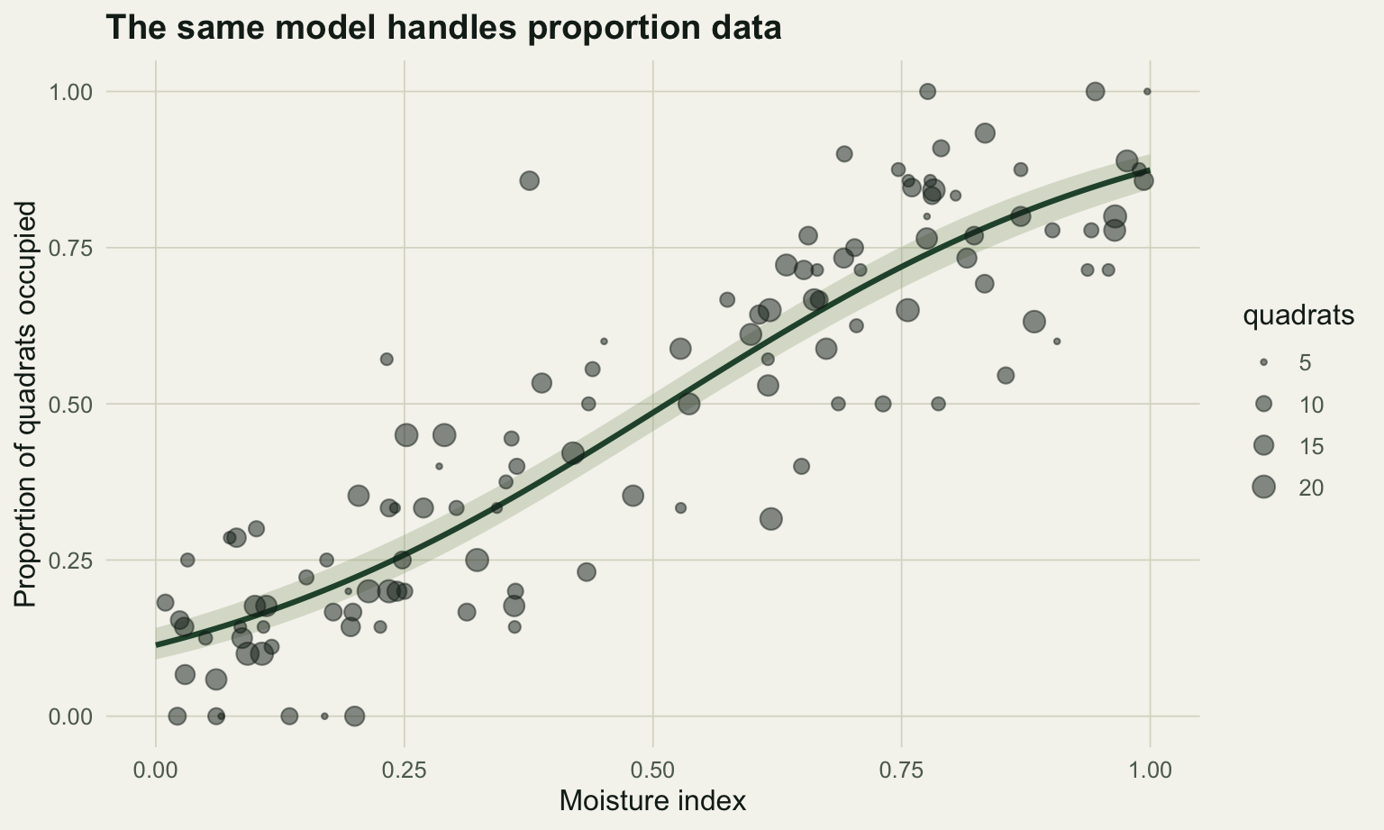
The binomial model is not only for single zeros and ones. If you visit each site and record how many of several quadrats are occupied, the response is a proportion, and the same family handles it. Pass the counts as a two-column matrix of successes and failures rather than as a raw fraction.
```{r}
set.seed(74)
ns <- 120
moisture <- runif(ns, 0, 1)
nq <- sample(5:20, ns, replace = TRUE)        # quadrats per site, unequal
k  <- rbinom(ns, nq, plogis(-2 + 4 * moisture))

m2 <- glm(cbind(k, nq - k) ~ moisture, family = binomial)
round(summary(m2)$coefficients, 3)
```
The fit recovers the generating values closely (intercept near -2, slope near 4). The two-column response matters because it carries the sample size: a site with 20 quadrats occupied 18 times is stronger evidence than a site with 5 quadrats occupied 4 times, even though both proportions are similar, and the model weights them accordingly. Collapsing to a raw fraction throws that away.
```{r}
# the wrong way: a linear model on raw proportions
round(coef(lm(I(k / nq) ~ moisture))[2], 3)
```
A linear model on the raw proportions returns a slope of 0.842, which is not even on the same scale as the GLM coefficient and ignores both the unequal sample sizes and the bounded 0-to-1 response. The older habit of an arcsine square-root transformation has the same interpretability problem and can produce predictions outside the valid range; for binomial data, logistic regression has both clearer meaning and more power, and the transformation is best treated as a historical relic (Warton and Hui 2011). If the proportions show more scatter than the binomial allows, that is overdispersion, and the fix is a random effect, which is the subject of the GLMM post rather than a reason to transform.
```{r}
#| label: fig-prop
#| fig-cap: "Proportion of quadrats occupied against moisture, with point size showing the number of quadrats per site and the fitted binomial curve."
#| fig-alt: "Scatter of occupied-quadrat proportions rising with moisture; larger points carry more quadrats, and a green logistic curve with a narrow band runs through them."
#| fig-width: 8
#| fig-height: 4.8
#| message: false
#| warning: false
xx2 <- data.frame(moisture = seq(0, 1, length = 200))
pr2 <- predict(m2, xx2, type = "link", se.fit = TRUE)
xx2$fit <- plogis(pr2$fit)
xx2$lo  <- plogis(pr2$fit - 1.96 * pr2$se.fit)
xx2$hi  <- plogis(pr2$fit + 1.96 * pr2$se.fit)

ggplot() +
  geom_ribbon(data = xx2, aes(moisture, ymin = lo, ymax = hi), fill = sage, alpha = .3) +
  geom_line(data = xx2, aes(moisture, fit), colour = forest, linewidth = 1.1) +
  geom_point(data = data.frame(moisture, prop = k / nq, nq),
             aes(moisture, prop, size = nq), alpha = .5, colour = ink) +
  scale_size_continuous(range = c(.8, 4), name = "quadrats") +
  labs(x = "Moisture index", y = "Proportion of quadrats occupied",
       title = "The same model handles proportion data") +
  te_theme
```
## The separation trap
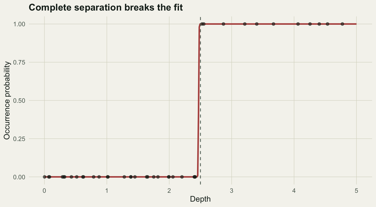
One failure mode is worth recognising on sight, because the model does not always announce it clearly. If a predictor perfectly splits presences from absences, the maximum likelihood estimate does not exist: the likelihood keeps increasing as the coefficient grows without bound, so the fitting algorithm never settles.
```{r}
set.seed(11)
nsep <- 40
depth <- sort(runif(nsep, 0, 5))
occ <- as.integer(depth > 2.5)            # depth predicts occurrence perfectly
msep <- glm(occ ~ depth, family = binomial)
```
The warning is the first clue. The coefficient is the second.
```{r}
round(summary(msep)$coefficients["depth", c("Estimate", "Std. Error")], 1)
range(fitted(msep))
```
The slope has run off to roughly 344 with a standard error in the tens of thousands, and the fitted probabilities are pinned at exactly 0 and 1. These are the fingerprints of complete separation. Albert and Anderson (1984) classified the patterns precisely: with overlap the usual estimates exist, but under complete or quasi-complete separation the finite maximum likelihood estimate does not, and the standard errors are meaningless. The number is not a strong effect; it is a non-answer.
The remedy is not to trust the output. Penalised likelihood (Firth's method, in the `logistf` package) keeps the estimates finite and is the standard fix. Often the more useful response is to ask why a predictor separates the data perfectly: with a small sample it can happen by chance, and with a strong predictor it can signal that the question is really about a threshold rather than a smooth gradient.
```{r}
#| label: fig-sep
#| fig-cap: "Complete separation: depth predicts occurrence perfectly, so the fitted curve collapses to a vertical step and the coefficient diverges."
#| fig-alt: "Occurrence points are all zero below a depth of 2.5 and all one above it; the fitted red curve is a vertical step at that threshold rather than a smooth S-curve."
#| fig-width: 8
#| fig-height: 4.4
#| message: false
#| warning: false
xx3 <- data.frame(depth = seq(0, 5, length = 400))
xx3$fit <- predict(msep, xx3, type = "response")
ggplot() +
  geom_line(data = xx3, aes(depth, fit), colour = accent, linewidth = 1.1) +
  geom_point(data = data.frame(depth, occ), aes(depth, occ),
             alpha = .6, colour = ink, size = 1.8) +
  geom_vline(xintercept = 2.5, linetype = "dashed", colour = "#5d6b61") +
  labs(x = "Depth", y = "Occurrence probability",
       title = "Complete separation breaks the fit") +
  te_theme
```
## Where this fits
The binomial GLM is the binary sibling of the [count GLM](../glm-count-data-abundance/): same iteratively reweighted least squares underneath, different link and distribution chosen to match the response. It is also the modelling end of the spatial-data workflow. The [terra raster post](../terra-raster-basics/) extracts environmental values at species occurrence points; feed those values and a presence-absence column into a binomial GLM and you have a simple species distribution model. When the binary or proportion data are grouped, with repeated visits to the same sites, the independence assumption breaks and the model needs a random effect, exactly as in the [GLMM post](../glmm-nested-counts-pseudoreplication/).
## References
Albert & Anderson 1984 Biometrika 71(1):1-10 (10.1093/biomet/71.1.1)
Guisan & Zimmermann 2000 Ecological Modelling 135(2-3):147-186 (10.1016/S0304-3800(00)00354-9)
McCullagh & Nelder 1989 Generalized Linear Models, 2nd edition, Chapman and Hall (ISBN 0-412-31760-5)
Nelder & Wedderburn 1972 Journal of the Royal Statistical Society A 135(3):370-384 (10.2307/2344614)
Warton & Hui 2011 Ecology 92(1):3-10 (10.1890/10-0340.1)