Class imbalance in species presence models

What class imbalance does to a species presence model in R: why the positive count and not the ratio limits the fit, and what downsampling really changes.

You survey 4000 sites, find the species at 105 of them, fit a logistic regression, and the model predicts absence everywhere. Someone tells you the data are imbalanced and that you should downsample the absences, or upsample the presences, or set class weights. The advice is everywhere in the applied machine learning literature and it has moved wholesale into species distribution work, usually without anyone measuring what it does.

This tutorial measures it. The claim I want to establish is sharper than “imbalance breaks the model”, because that claim is close to false. What limits a rare species model is the number of presences, not the ratio of presences to absences. The ranking of sites by predicted suitability is barely affected by imbalance at all. Two things do break: the default rule of calling a site occupied when the predicted probability passes 0.5, and, after you apply the usual remedy, the meaning of the predicted probabilities themselves.

Everything is simulated, so the truth is known and the arithmetic can be checked against it. The measurements are: the standard error of a slope under two designs that separate the ratio from the count; how many sites a correctly specified model calls occupied at 0.5 while its AUC sits near 0.85; the exact intercept shift that downsampling produces, verified against the analytic value; a scoreboard of five remedies at four prevalences; and one regime where a small presence count genuinely destroys an estimate. If you want the mechanics of fitting the model in the first place, that is in Logistic regression for presence-absence data.

library(ggplot2)

te_pal <- list(forest = "#275139", green = "#2f8f63", sage = "#93a87f",
               clay = "#b5534e", gold = "#cda23f", line = "#dad9ca",
               ink = "#16241d", paper = "#f5f4ee")

theme_te <- function() {
  theme_minimal(base_size = 12) +
    theme(panel.grid.minor = element_blank(),
          panel.grid.major = element_line(colour = "#e7e6dc"),
          plot.background = element_rect(fill = "#f5f4ee", colour = NA),
          panel.background = element_rect(fill = "#f5f4ee", colour = NA),
          plot.title = element_text(face = "bold", colour = te_pal$ink),
          axis.title = element_text(colour = "#2c3a31"))
}

One generative model for the whole post

Every dataset below comes from the same three coefficients: an intercept of -4.6, an elevation slope of 1.3 and a wetness slope of -0.9, both predictors standard normal and independent. That intercept puts the occupancy probability at an average site at 0.0100, and averaging the curve over the predictors lifts the marginal prevalence to 0.0282, because the logistic curve is convex in this region and the good sites contribute more than the bad ones take away.

set.seed(20260815)
b_int <- -4.6; b_elev <- 1.3; b_wet <- -0.9

sim_sites <- function(nn, b0 = b_int) {
  ev <- rnorm(nn); wv <- rnorm(nn)
  data.frame(elev = ev, wet = wv,
             occ = rbinom(nn, 1, plogis(b0 + b_elev * ev + b_wet * wv)))
}

auc_of <- function(score, yy) {
  rk <- rank(score)
  n1 <- sum(yy == 1); n0 <- sum(yy == 0)
  (sum(rk[yy == 1]) - n1 * (n1 + 1) / 2) / (n1 * n0)
}

check <- sim_sites(200000)
cat(sprintf("true coefficients: intercept %.1f, elevation %.1f, wetness %.1f\n",
            b_int, b_elev, b_wet))

true coefficients: intercept -4.6, elevation 1.3, wetness -0.9

cat(sprintf("marginal prevalence from 200000 sites: %.4f\n", mean(check$occ)))

marginal prevalence from 200000 sites: 0.0282

cat(sprintf("occupancy probability at an average site: %.4f\n", plogis(b_int)))

occupancy probability at an average site: 0.0100

The model is correctly specified throughout: the fitted equation is the equation that generated the data. That is a strong assumption and the last section says what it hides.

The ratio is not the problem, the count is

“Imbalance” names a ratio. To find out whether the ratio is what hurts, hold it against the count in two designs drawn from the same pool of 1200000 sites. Design A fixes the number of presences at 60 and adds absences, so the prevalence in the sample falls from 0.5 to 0.0030 while the presence count never changes. Design B fixes the prevalence at 0.03 and grows the whole survey, so the presence count rises with it. In both, the quantity watched is the standard error of the elevation slope, averaged over replicate draws.

set.seed(11235)
n_pop <- 1200000
pop <- sim_sites(n_pop)
pos_all <- which(pop$occ == 1)
neg_all <- which(pop$occ == 0)
cat(sprintf("pool: %d sites, %d occupied, prevalence %.4f\n",
            n_pop, length(pos_all), mean(pop$occ)))

pool: 1200000 sites, 34412 occupied, prevalence 0.0287

n_warn <- 0
se_slope <- function(rows) {
  fit <- withCallingHandlers(
    glm(occ ~ elev + wet, data = pop[rows, ], family = binomial),
    warning = function(w) { n_warn <<- n_warn + 1; invokeRestart("muffleWarning") })
  summary(fit)$coefficients["elev", "Std. Error"]
}

The warning counter is there because a small presence count is exactly the situation in which a logistic fit can fail quietly. Nothing is being hidden: the count is printed with the results.

n_fix <- 60
neg_grid <- c(60, 180, 600, 1800, 6000, 20000)
rep_a <- 60
se_a <- vapply(neg_grid, function(nn)
  mean(replicate(rep_a, se_slope(c(sample(pos_all, n_fix), sample(neg_all, nn))))),
  numeric(1))
tab_a <- data.frame(sites = n_fix + neg_grid, positives = n_fix,
                    prevalence = n_fix / (n_fix + neg_grid), se_elev = se_a)

prev_fix <- 0.03
tot_grid <- c(1000, 3000, 10000, 30000, 60000)
rep_b <- 30
se_b <- vapply(tot_grid, function(nn) {
  np <- round(nn * prev_fix)
  mean(replicate(rep_b, se_slope(c(sample(pos_all, np), sample(neg_all, nn - np)))))
}, numeric(1))
tab_b <- data.frame(sites = tot_grid, positives = round(tot_grid * prev_fix),
                    prevalence = prev_fix, se_elev = se_b)

cat(sprintf("design A: %d positives held fixed, %d replicate draws per grid point\n",
            n_fix, rep_a))

design A: 60 positives held fixed, 60 replicate draws per grid point

print(round(tab_a, 4))

  sites positives prevalence se_elev
1   120        60     0.5000  0.2852
2   240        60     0.2500  0.2239
3   660        60     0.0909  0.1806
4  1860        60     0.0323  0.1583
5  6060        60     0.0099  0.1470
6 20060        60     0.0030  0.1415

cat(sprintf("design B: prevalence held at %.2f, %d replicate draws per grid point\n",
            prev_fix, rep_b))

design B: prevalence held at 0.03, 30 replicate draws per grid point

print(round(tab_b, 4))

  sites positives prevalence se_elev
1  1000        30       0.03  0.2262
2  3000        90       0.03  0.1297
3 10000       300       0.03  0.0699
4 30000       900       0.03  0.0403
5 60000      1800       0.03  0.0286

cat(sprintf("glm warnings during both sweeps: %d\n", n_warn))

glm warnings during both sweeps: 0

Design A drives the prevalence down by a factor of more than one hundred and sixty and the standard error gets better, from 0.2852 to 0.1415. Whatever imbalance is doing, it is not punishing the fit for being imbalanced. Design B holds the prevalence at a fixed 0.03, which by the usual telling should keep the problem constant, and the standard error falls from 0.2262 to 0.0286.

cat(sprintf("exponent on positives, fixed prevalence: %.4f\n",
            coef(lm(log(se_b) ~ log(tab_b$positives)))[2]))

exponent on positives, fixed prevalence: -0.5060

cat(sprintf("exponent on negatives, fixed positives:  %.4f\n",
            coef(lm(log(se_a) ~ log(neg_grid)))[2]))

exponent on negatives, fixed positives:  -0.1201

cat(sprintf("fixed positives: se %.4f to %.4f, a %.3f-fold gain for %.0f times the absences\n",
            se_a[1], se_a[6], se_a[1] / se_a[6], neg_grid[6] / neg_grid[1]))

fixed positives: se 0.2852 to 0.1415, a 2.016-fold gain for 333 times the absences

cat(sprintf("last step of design A: %d to %d absences cuts the se by %.1f percent\n",
            neg_grid[5], neg_grid[6], 100 * (1 - se_a[6] / se_a[5])))

last step of design A: 6000 to 20000 absences cuts the se by 3.8 percent

cat(sprintf("%d sites with %d positives: se %.4f\n", tab_a$sites[6], n_fix, se_a[6]))

20060 sites with 60 positives: se 0.1415

cat(sprintf("%d sites with %d positives: se %.4f (ratio %.2f)\n",
            tab_b$sites[3], tab_b$positives[3], se_b[3], se_a[6] / se_b[3]))

10000 sites with 300 positives: se 0.0699 (ratio 2.03)

Fit a power law to each sweep and the two designs separate cleanly. Against the number of presences at fixed prevalence the exponent is -0.5060, which is the textbook inverse square root: quadruple your presences and the standard error halves. Against the number of absences at a fixed presence count the exponent is -0.1201, and it is not even a real power law, because the curve is flattening towards a floor rather than descending. Going from 60 absences to 20000, a rise of 333-fold, buys a 2.016-fold improvement in total, and the last leg of that journey, from 6000 absences to 20000, is worth 3.8 percent.

The comparison that matters for a survey design is the last pair of lines. A sample of 20060 sites carrying 60 presences gives a standard error of 0.1415. A sample of 10000 sites, half the fieldwork, carrying 300 presences gives 0.0699, better by a factor of 2.03. Sites are not the currency. Presences are.

sweep_dat <- rbind(
  data.frame(tab_a, design = "60 positives, absences added"),
  data.frame(tab_b, design = "prevalence 0.03, survey grows"))

p_se <- ggplot(sweep_dat, aes(sites, se_elev, colour = design)) +
  geom_line(linewidth = 0.9) +
  geom_point(size = 2.4) +
  scale_x_log10() +
  scale_y_log10() +
  scale_colour_manual(values = c(te_pal$clay, te_pal$forest)) +
  labs(title = "Only the positives buy precision",
       x = "sites in the sample (log scale)",
       y = "standard error of the elevation slope (log scale)",
       colour = NULL) +
  theme_te() +
  theme(legend.position = "top")
print(p_se)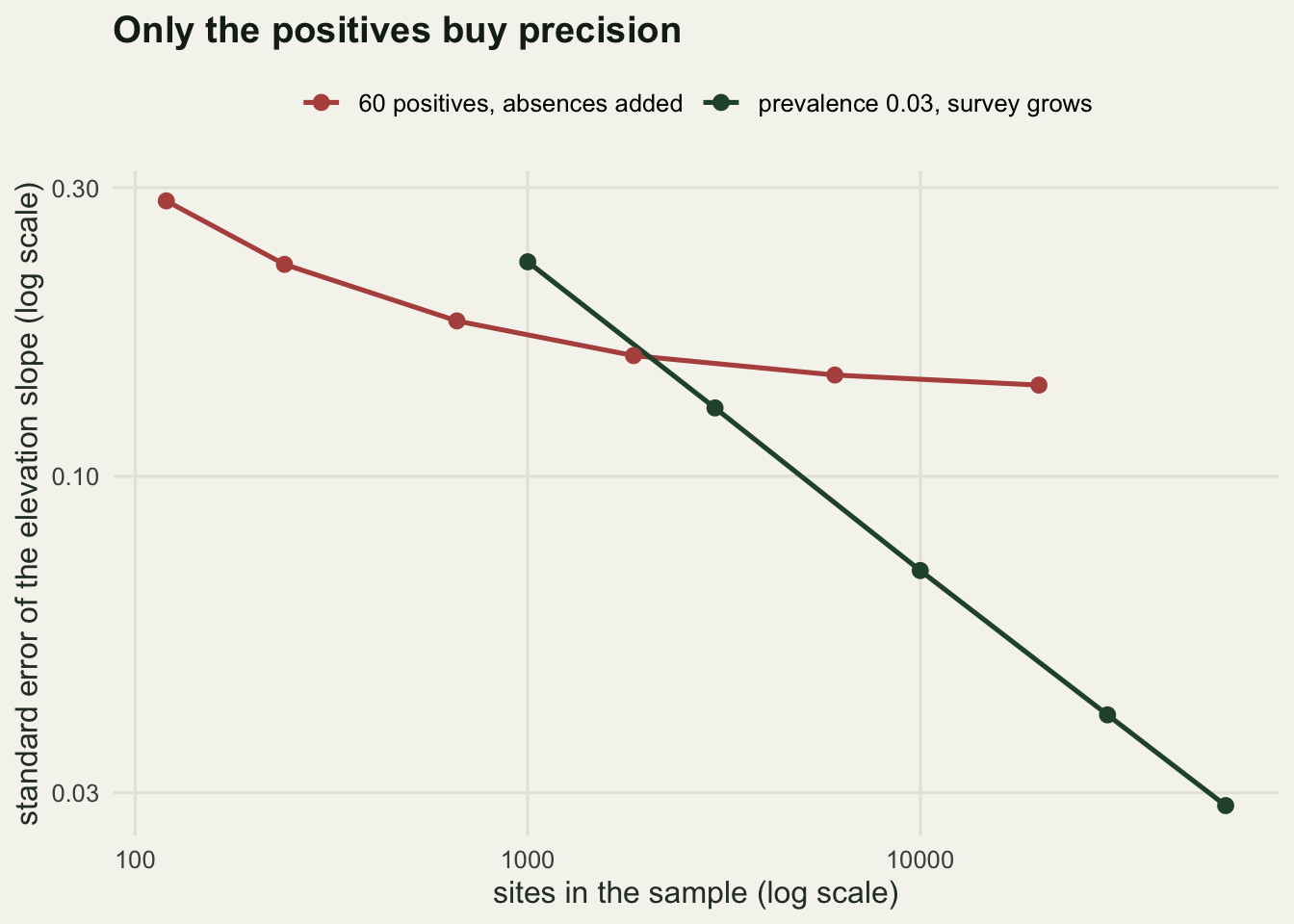

Standard error of the elevation slope against sample size under two designs. Holding the presence count at 60 and adding absences flattens out; holding prevalence at 0.03 and growing the survey keeps descending on the inverse square root line.

Adding absences is not useless. The first few hundred sharpen the picture of what an unoccupied site looks like, which is why the curve drops at the left. Past a ratio of about one hundred absences per presence, the absences have told you everything they are going to tell you about the background, and the remaining uncertainty is all about the small pile of presences.

The model that never calls a site occupied

Now take a single survey of the size an ecologist actually walks: 4000 sites at the prevalence above. Fit the model, and apply the rule that every classifier tutorial applies by default, which is to call a site occupied when the predicted probability is at least 0.5.

set.seed(4142)
survey <- sim_sites(4000)
fit_sv <- glm(occ ~ elev + wet, data = survey, family = binomial)
p_hat <- fitted(fit_sv)
called <- p_hat >= 0.5
cat(sprintf("survey: %d sites, %d occupied, prevalence %.4f\n",
            nrow(survey), sum(survey$occ), mean(survey$occ)))

survey: 4000 sites, 105 occupied, prevalence 0.0262

print(round(summary(fit_sv)$coefficients, 4))

            Estimate Std. Error  z value Pr(>|z|)
(Intercept)  -4.5554     0.1729 -26.3501        0
elev          1.2285     0.1125  10.9171        0
wet          -0.7855     0.1062  -7.3931        0

cat(sprintf("largest fitted probability: %.4f\n", max(p_hat)))

largest fitted probability: 0.6788

cat(sprintf("sites called present at 0.5: %d, of which really occupied: %d\n",
            sum(called), sum(called & survey$occ == 1)))

sites called present at 0.5: 4, of which really occupied: 3

The coefficients are fine. An intercept of -4.5554 against a true -4.6, an elevation slope of 1.2285 against a true 1.3, a wetness slope of -0.7855 against a true -0.9: all three within about one standard error of the truth. The model has learned the ecology. It also calls exactly 4 of the 4000 sites occupied, and only 3 of those 4 really are, against 105 occupied sites in the data. The largest fitted probability anywhere in the survey is 0.6788, so only a handful of sites can clear the bar no matter how the labels fall.

sens <- sum(called & survey$occ == 1) / sum(survey$occ == 1)
spec <- sum(!called & survey$occ == 0) / sum(survey$occ == 0)
cat(sprintf("sensitivity %.4f, specificity %.4f, TSS %.4f\n", sens, spec, sens + spec - 1))

sensitivity 0.0286, specificity 0.9997, TSS 0.0283

cat(sprintf("accuracy of the 0.5 rule: %.4f\n", mean(called == (survey$occ == 1))))

accuracy of the 0.5 rule: 0.9742

cat(sprintf("accuracy of calling every site absent: %.4f\n", mean(survey$occ == 0)))

accuracy of calling every site absent: 0.9738

cat(sprintf("AUC of the same fitted values: %.4f\n", auc_of(p_hat, survey$occ)))

AUC of the same fitted values: 0.8388

cat(sprintf("median fitted probability, occupied %.4f, empty %.4f\n",
            median(p_hat[survey$occ == 1]), median(p_hat[survey$occ == 0])))

median fitted probability, occupied 0.0615, empty 0.0098

Sensitivity is 0.0286 and specificity is 0.9997, so the true skill statistic is 0.0283, near enough to the score of a rule that ignores the data. The accuracy of the 0.5 rule is 0.9742 against 0.9738 for a script that prints “absent” 4000 times, a gain of four sites in four thousand. And the AUC of the very same fitted values is 0.8388.

That pair of numbers is the point of this section. The AUC says the model separates occupied from empty sites well: the median fitted probability is 0.0615 at an occupied site and 0.0098 at an empty one, more than a six-fold difference in the right direction. The confusion matrix at 0.5 says the model is useless. Both are correct, and they are answering different questions. AUC is a statement about ranking, computed within the occupied sites and within the empty ones separately. The 0.5 rule is a statement about where the probability scale crosses a fixed line that has nothing to do with this species.

prob_dat <- data.frame(p_hat = p_hat,
                       state = ifelse(survey$occ == 1, "occupied", "empty"))
p_prob <- ggplot(prob_dat, aes(p_hat, fill = state, colour = state)) +
  geom_histogram(bins = 40, position = "identity", alpha = 0.45) +
  geom_vline(xintercept = 0.5, linetype = "dashed", colour = te_pal$ink) +
  scale_x_log10() +
  scale_y_sqrt() +
  scale_fill_manual(values = c(te_pal$sage, te_pal$clay)) +
  scale_colour_manual(values = c(te_pal$sage, te_pal$clay)) +
  labs(title = "The fitted probabilities never reach the default rule",
       x = "fitted probability of presence (log scale)",
       y = "sites (square root scale)", fill = NULL, colour = NULL) +
  theme_te() +
  theme(legend.position = "top")
print(p_prob)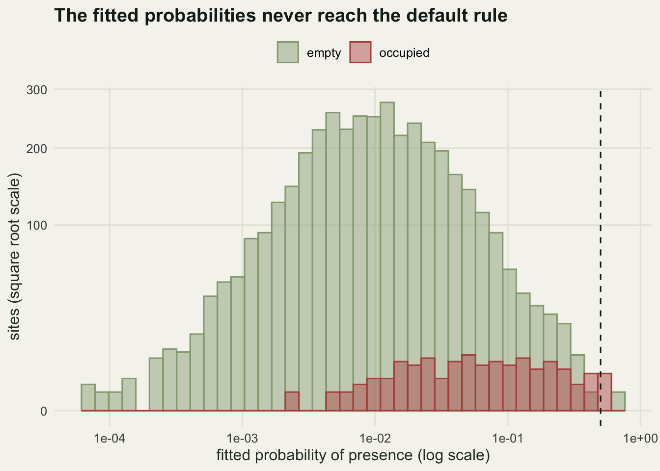

Fitted probabilities from the 4000 site survey, split by true occupancy. The distributions are well separated on the log scale, and both sit far below the dashed 0.5 line.

A rare species is rare. A well-fitted model of a rare species should predict low probabilities nearly everywhere, and 0.5 is not a probability that a 3 percent species has any business reaching outside a few exceptional sites. The rule is broken, not the model.

What downsampling does, exactly

The standard remedy is to throw away most of the absences so that the two classes are balanced. This has a closed form, and it is old: it is the case-control result from epidemiology, restated for anyone who samples the two outcome classes at different rates. If you keep a fraction of the presences and a fraction of the absences, the logistic coefficients you get back are the population coefficients with one change, an intercept shifted by the log of the ratio of the two sampling fractions. The slopes are untouched.

Take an atlas of 40000 grid squares, fit the full model, then keep every occupied square and a random equal number of empty ones.

set.seed(2718)
atlas <- sim_sites(40000)
pos_r <- which(atlas$occ == 1)
neg_r <- which(atlas$occ == 0)
n_pos <- length(pos_r); n_neg <- length(neg_r)
cat(sprintf("atlas: %d squares, %d occupied, %d empty, prevalence %.4f\n",
            nrow(atlas), n_pos, n_neg, mean(atlas$occ)))

atlas: 40000 squares, 1117 occupied, 38883 empty, prevalence 0.0279

fit_full <- glm(occ ~ elev + wet, data = atlas, family = binomial)
fit_down <- glm(occ ~ elev + wet, data = atlas[c(pos_r, sample(neg_r, n_pos)), ],
                family = binomial)
frac_1 <- 1
frac_0 <- n_pos / n_neg
off_an <- log(frac_1 / frac_0)
side <- cbind(full = coef(fit_full), downsampled = coef(fit_down),
              difference = coef(fit_down) - coef(fit_full))
print(round(side, 4))

               full downsampled difference
(Intercept) -4.6731     -1.0667     3.6064
elev         1.3449      1.2744    -0.0704
wet         -0.8943     -0.8823     0.0120

cat(sprintf("sampling fractions: presences %.4f, absences %.4f\n", frac_1, frac_0))

sampling fractions: presences 1.0000, absences 0.0287

cat(sprintf("analytic intercept offset log(%.4f / %.4f) = %.4f\n", frac_1, frac_0, off_an))

analytic intercept offset log(1.0000 / 0.0287) = 3.5499

cat(sprintf("measured intercept difference %.4f, gap %.4f\n",
            side["(Intercept)", "difference"], side["(Intercept)", "difference"] - off_an))

measured intercept difference 3.6064, gap 0.0565

cat(sprintf("slope gaps in units of the downsampled standard error: elev %.3f, wet %.3f\n",
            side["elev", "difference"] / summary(fit_down)$coefficients["elev", "Std. Error"],
            side["wet", "difference"] / summary(fit_down)$coefficients["wet", "Std. Error"]))

slope gaps in units of the downsampled standard error: elev -1.140, wet 0.200

The intercept goes from -4.6731 to -1.0667, a jump of 3.6064. The analytic prediction, the log of 1 over the absence sampling fraction of 0.0287, is 3.5499. The gap is 0.0565. The elevation slope moves from 1.3449 to 1.2744 and the wetness slope from -0.8943 to -0.8823, which is 1.140 and 0.200 standard errors of the downsampled fit: noise, in the direction of nothing in particular.

One draw is one draw, so repeat the downsampling and look at the spread.

n_rep <- 200
draw_down <- function() {
  glm(occ ~ elev + wet, data = atlas[c(pos_r, sample(neg_r, n_pos)), ], family = binomial)
}
rep_coef <- t(replicate(n_rep, coef(draw_down())))
cat(sprintf("downsampling repeated %d times\n", n_rep))

downsampling repeated 200 times

print(round(rbind(mean = colMeans(rep_coef), sd = apply(rep_coef, 2, sd),
                  full_data = coef(fit_full)), 4))

          (Intercept)   elev     wet
mean          -1.0913 1.2801 -0.9162
sd             0.0201 0.0418  0.0422
full_data     -4.6731 1.3449 -0.8943

cat(sprintf("mean intercept shift %.4f against analytic %.4f (gap %.4f, full-fit se %.4f)\n",
            mean(rep_coef[, 1]) - coef(fit_full)[1], off_an,
            mean(rep_coef[, 1]) - coef(fit_full)[1] - off_an,
            summary(fit_full)$coefficients[1, "Std. Error"]))

mean intercept shift 3.5818 against analytic 3.5499 (gap 0.0319, full-fit se 0.0577)

Over 200 downsamples the mean intercept shift is 3.5818 against an analytic 3.5499, a residual of 0.0319 that is a little over half the standard error of the full-data intercept itself, 0.0577. The slopes average 1.2801 and -0.9162 against the full-data 1.3449 and -0.8943, with resampling standard deviations of 0.0418 and 0.0422. The identity is not exact in a finite sample, and I would not want to claim otherwise: maximum likelihood logistic coefficients carry a small-sample bias away from zero, and a balanced subsample of 1117 pairs is a smaller sample than the atlas it came from. The identity is exact in the limit and close enough here that the intercept shift is predictable to two decimal places before you run anything.

Now score the two models out of sample.

set.seed(3141)
holdout <- sim_sites(40000)
lp_down <- predict(fit_down, holdout)
pr_full <- predict(fit_full, holdout, type = "response")
pr_down <- plogis(lp_down)
pr_corr <- plogis(lp_down - off_an)
brier_of <- function(pv, yy) mean((pv - yy)^2)
cox_of <- function(pv, yy) coef(glm(yy ~ qlogis(pv), family = binomial))
score_tab <- data.frame(
  auc = c(auc_of(pr_full, holdout$occ), auc_of(pr_down, holdout$occ),
          auc_of(pr_corr, holdout$occ)),
  brier = c(brier_of(pr_full, holdout$occ), brier_of(pr_down, holdout$occ),
            brier_of(pr_corr, holdout$occ)),
  mean_pred = c(mean(pr_full), mean(pr_down), mean(pr_corr)),
  cal_int = c(cox_of(pr_full, holdout$occ)[1], cox_of(pr_down, holdout$occ)[1],
              cox_of(pr_corr, holdout$occ)[1]),
  cal_slope = c(cox_of(pr_full, holdout$occ)[2], cox_of(pr_down, holdout$occ)[2],
                cox_of(pr_corr, holdout$occ)[2]),
  row.names = c("full data", "downsampled", "downsampled, offset removed"))
cat(sprintf("held-out squares: %d, observed prevalence %.4f\n",
            nrow(holdout), mean(holdout$occ)))

held-out squares: 40000, observed prevalence 0.0290

print(round(score_tab, 5))

                                auc   brier mean_pred  cal_int cal_slope
full data                   0.85281 0.02517   0.02750 -0.00142   0.97752
downsampled                 0.85265 0.15590   0.32218 -3.48305   1.01847
downsampled, offset removed 0.85265 0.02518   0.02696  0.13242   1.01847

cat(sprintf("Brier ratio, downsampled over full: %.2f\n",
            score_tab$brier[2] / score_tab$brier[1]))

Brier ratio, downsampled over full: 6.19

cat(sprintf("calibration intercept of the downsampled fit %.4f against offset %.4f\n",
            score_tab$cal_int[2], -off_an))

calibration intercept of the downsampled fit -3.4831 against offset -3.5499

The calibration measure here is the pair of coefficients from regressing the held-out outcome on the logit of the prediction. A model whose probabilities mean what they say returns an intercept of 0 and a slope of 1.

Read the table row by row. AUC is 0.85281 for the full model and 0.85265 for the downsampled one; the difference is in the fourth decimal and comes from the slightly different slopes, since an intercept change cannot alter a ranking at all. The Brier score goes from 0.02517 to 0.15590, worse by a factor of 6.19. The mean predicted probability goes from 0.02750, which is the observed prevalence of 0.0290 to within sampling noise, to 0.32218, which is nothing at all: it is the prevalence of the subsample that was fitted, not of the landscape. The calibration intercept goes from -0.00142 to -3.48305, and that number is the offset back again, up to the same finite-sample slack as before.

Subtract the analytic offset from the linear predictor and the third row shows what comes back. AUC is identical to the downsampled model, to every digit, because subtracting a constant on the logit scale is a monotone transformation. The Brier score returns to 0.02518, a hair above the full model’s 0.02517. The calibration intercept lands at 0.13242 rather than 0, the leftover of the same finite-sample gap.

n_bin <- 8
brk <- quantile(pr_full, seq(0, 1, length.out = n_bin + 1))
which_bin <- cut(pr_full, brk, include.lowest = TRUE, labels = FALSE)
obs_rate <- tapply(holdout$occ, which_bin, mean)
bin_dat <- rbind(
  data.frame(model = "full data", pred = tapply(pr_full, which_bin, mean), obs = obs_rate),
  data.frame(model = "downsampled", pred = tapply(pr_down, which_bin, mean), obs = obs_rate),
  data.frame(model = "downsampled, offset removed",
             pred = tapply(pr_corr, which_bin, mean), obs = obs_rate))
cat(sprintf("bins of %d squares; empty bins dropped: %d\n",
            nrow(holdout) / n_bin, sum(obs_rate == 0)))

bins of 5000 squares; empty bins dropped: 0

print(round(data.frame(predicted = tapply(pr_full, which_bin, mean),
                       downsampled = tapply(pr_down, which_bin, mean),
                       observed = obs_rate), 5))

  predicted downsampled observed
1   0.00078     0.03057   0.0012
2   0.00225     0.08053   0.0026
3   0.00433     0.14151   0.0050
4   0.00738     0.21583   0.0064
5   0.01218     0.30863   0.0146
6   0.02072     0.42718   0.0204
7   0.03902     0.57912   0.0414
8   0.13332     0.79410   0.1400

bin_dat <- bin_dat[bin_dat$obs > 0, ]

p_cal <- ggplot(bin_dat, aes(pred, obs, colour = model)) +
  geom_abline(intercept = 0, slope = 1, linetype = "dashed", colour = te_pal$ink) +
  geom_line(linewidth = 0.9) +
  geom_point(size = 2.4) +
  scale_x_log10() +
  scale_y_log10() +
  scale_colour_manual(values = c(te_pal$clay, te_pal$gold, te_pal$forest)) +
  labs(title = "Downsampling moves the probabilities, not the ranking",
       x = "mean predicted probability in the bin (log scale)",
       y = "observed occupancy in the bin (log scale)", colour = NULL) +
  theme_te() +
  theme(legend.position = "top")
print(p_cal)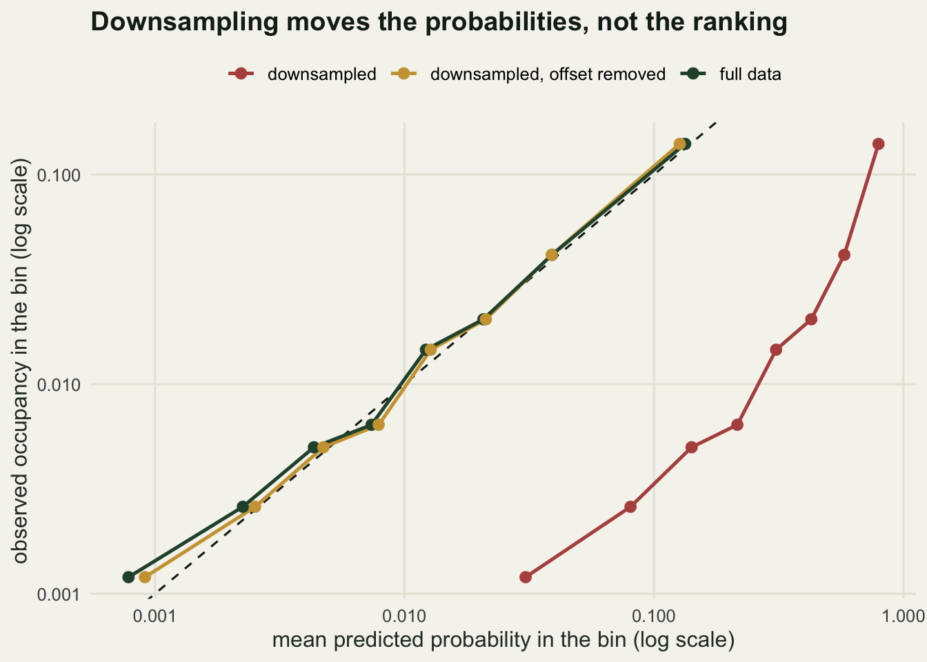

Calibration of the three models on 40000 held-out squares, in eight bins of equal size. The full model and the offset-corrected model sit on the diagonal; the downsampled model is displaced upward by more than an order of magnitude at the low end.

The bin table is the same story without the model fitting. In the lowest eighth of the atlas the observed occupancy is 0.0012 and the full model predicts 0.00078, while the downsampled model predicts 0.03057. In the top eighth the observed occupancy is 0.1400, the full model says 0.13332 and the downsampled model says 0.79410. A square where the species turns up in one visit out of seven is being reported as almost certain habitat.

That is the whole of what downsampling did. It multiplied the odds everywhere by a constant and left the ecology alone.

Scoring the remedies against doing nothing

Downsampling is one of three remedies in circulation. Upsampling draws presences with replacement until the classes are balanced; class weights give each presence a weight equal to the ratio of absences to presences and fit on the whole dataset. Put all three next to the raw model at 0.5 and the raw model at a threshold tuned on the training data, at four prevalences from a third of sites occupied down to two percent. The threshold is tuned by maximising the true skill statistic on the training data, which is the ordinary practice in species distribution work.

set.seed(1618)
tss_at <- function(pv, yy, thr) {
  sum(pv >= thr & yy == 1) / sum(yy == 1) + sum(pv < thr & yy == 0) / sum(yy == 0) - 1
}
tss_max <- function(pv, yy) {
  o <- order(-pv); ys <- yy[o]
  max(cumsum(ys) / sum(ys) - cumsum(1 - ys) / sum(1 - ys))
}
tune_thr <- function(pv, yy) {
  cand <- sort(unique(round(pv, 4)))
  cand[which.max(vapply(cand, function(tt) tss_at(pv, yy, tt), numeric(1)))]
}

b0_grid <- c(-1.0, -2.2, -3.4, -4.6)
n_train <- 4000
n_test <- 40000

one_prevalence <- function(b0) {
  tr <- sim_sites(n_train, b0)
  te <- sim_sites(n_test, b0)
  ip <- which(tr$occ == 1); iq <- which(tr$occ == 0)
  m_raw <- glm(occ ~ elev + wet, data = tr, family = binomial)
  m_down <- glm(occ ~ elev + wet, data = tr[c(ip, sample(iq, length(ip))), ],
                family = binomial)
  up_rows <- c(iq, sample(ip, length(iq), replace = TRUE))
  m_up <- glm(occ ~ elev + wet, data = tr[up_rows, ], family = binomial)
  wgt <- ifelse(tr$occ == 1, length(iq) / length(ip), 1)
  m_wt <- suppressWarnings(
    glm(occ ~ elev + wet, data = tr, family = binomial, weights = wgt))
  preds <- list(predict(m_raw, te, type = "response"), predict(m_raw, te, type = "response"),
                predict(m_down, te, type = "response"), predict(m_up, te, type = "response"),
                predict(m_wt, te, type = "response"))
  thrs <- c(0.5, tune_thr(fitted(m_raw), tr$occ), 0.5, 0.5, 0.5)
  data.frame(prevalence = mean(tr$occ), positives = sum(tr$occ),
             rule = c("raw, cut at 0.5", "raw, tuned cut", "downsampled, cut at 0.5",
                      "upsampled, cut at 0.5", "class weights, cut at 0.5"),
             cut_at = thrs,
             auc = vapply(preds, function(pv) auc_of(pv, te$occ), numeric(1)),
             brier = vapply(preds, function(pv) brier_of(pv, te$occ), numeric(1)),
             tss_used = mapply(function(pv, tt) tss_at(pv, te$occ, tt), preds, thrs),
             tss_best = vapply(preds, function(pv) tss_max(pv, te$occ), numeric(1)))
}
remedy_tab <- do.call(rbind, lapply(b0_grid, one_prevalence))
cat(sprintf("training sites %d, test sites %d, prevalences tested: %d\n",
            n_train, n_test, length(b0_grid)))

training sites 4000, test sites 40000, prevalences tested: 4

show_tab <- remedy_tab[, c("prevalence", "rule", "cut_at", "auc", "brier",
                           "tss_used", "tss_best")]
show_tab[, c(1, 3:7)] <- round(show_tab[, c(1, 3:7)], 4)
print(show_tab, row.names = FALSE)

 prevalence                      rule cut_at    auc  brier tss_used tss_best
     0.3365           raw, cut at 0.5 0.5000 0.8225 0.1575   0.4313   0.4899
     0.3365            raw, tuned cut 0.2988 0.8225 0.1575   0.4858   0.4899
     0.3365   downsampled, cut at 0.5 0.5000 0.8221 0.1730   0.4903   0.4905
     0.3365     upsampled, cut at 0.5 0.5000 0.8225 0.1737   0.4897   0.4901
     0.3365 class weights, cut at 0.5 0.5000 0.8225 0.1736   0.4886   0.4899
     0.1770           raw, cut at 0.5 0.5000 0.8306 0.1090   0.3174   0.4948
     0.1770            raw, tuned cut 0.2128 0.8306 0.1090   0.4896   0.4948
     0.1770   downsampled, cut at 0.5 0.5000 0.8300 0.1698   0.4902   0.4930
     0.1770     upsampled, cut at 0.5 0.5000 0.8302 0.1678   0.4890   0.4933
     0.1770 class weights, cut at 0.5 0.5000 0.8306 0.1683   0.4915   0.4947
     0.0727           raw, cut at 0.5 0.5000 0.8436 0.0580   0.0913   0.5210
     0.0727            raw, tuned cut 0.0765 0.8436 0.0580   0.5195   0.5210
     0.0727   downsampled, cut at 0.5 0.5000 0.8434 0.1706   0.5199   0.5217
     0.0727     upsampled, cut at 0.5 0.5000 0.8436 0.1631   0.5168   0.5221
     0.0727 class weights, cut at 0.5 0.5000 0.8437 0.1643   0.5177   0.5229
     0.0227           raw, cut at 0.5 0.5000 0.8492 0.0265   0.0162   0.5327
     0.0227            raw, tuned cut 0.0184 0.8492 0.0265   0.5287   0.5327
     0.0227   downsampled, cut at 0.5 0.5000 0.8492 0.1505   0.5273   0.5380
     0.0227     upsampled, cut at 0.5 0.5000 0.8495 0.1624   0.5260   0.5343
     0.0227 class weights, cut at 0.5 0.5000 0.8494 0.1599   0.5251   0.5349

rare <- remedy_tab[remedy_tab$prevalence == min(remedy_tab$prevalence), ]
cat(sprintf("at prevalence %.4f (%d positives):\n", rare$prevalence[1], rare$positives[1]))

at prevalence 0.0227 (91 positives):

cat(sprintf("  AUC spread across the five rules: %.5f\n", max(rare$auc) - min(rare$auc)))

  AUC spread across the five rules: 0.00026

cat(sprintf("  Brier, raw %.4f, resampled %.4f to %.4f\n",
            rare$brier[1], min(rare$brier[3:5]), max(rare$brier[3:5])))

  Brier, raw 0.0265, resampled 0.1505 to 0.1624

cat(sprintf("  TSS at the rule: raw at 0.5 %.4f, raw tuned %.4f, downsampled %.4f\n",
            rare$tss_used[1], rare$tss_used[2], rare$tss_used[3]))

  TSS at the rule: raw at 0.5 0.0162, raw tuned 0.5287, downsampled 0.5273

cat(sprintf("  best TSS available: raw %.4f, downsampled %.4f\n",
            rare$tss_best[1], rare$tss_best[3]))

  best TSS available: raw 0.5327, downsampled 0.5380

cat(sprintf("  tuned cut on the raw model: %.4f\n", rare$cut_at[2]))

  tuned cut on the raw model: 0.0184

At the rarest grid point, prevalence 0.0227 with 91 presences in the training data, the five rules span 0.00026 of AUC. That is the discrimination column and it is flat: none of the remedies improves the ranking, because none of them changes what the model knows about elevation and wetness. The Brier score goes the other way. The raw model scores 0.0265 and the three resampled fits score between 0.1505 and 0.1624, five to six times worse, for the reason the previous section made explicit.

The column people actually cite is the true skill statistic, and here the arithmetic is worth stating slowly. The raw model at 0.5 scores 0.0162. The downsampled model at 0.5 scores 0.5273. That is the entire published case for resampling, and it looks decisive. But the raw model at a threshold tuned on its own training data scores 0.5287, slightly better than the downsampled model, and the best true skill statistic available anywhere on the raw model’s ranking is 0.5327 against 0.5380 for the downsampled one. The tuned threshold is 0.0184, which is close to the prevalence, and that is not a coincidence: downsampling to balance is a threshold move dressed as a modelling choice, and the threshold it implies is roughly the prevalence.

long_dat <- rbind(
  data.frame(remedy_tab[, c("prevalence", "rule")], metric = "AUC",
             value = remedy_tab$auc),
  data.frame(remedy_tab[, c("prevalence", "rule")], metric = "Brier score",
             value = remedy_tab$brier),
  data.frame(remedy_tab[, c("prevalence", "rule")], metric = "TSS at the rule used",
             value = remedy_tab$tss_used))
long_dat$rule <- factor(long_dat$rule, levels = unique(remedy_tab$rule))
p_rem <- ggplot(long_dat, aes(prevalence, value, colour = rule, shape = rule)) +
  geom_line(linewidth = 0.8) +
  geom_point(size = 2.6) +
  facet_wrap(~ metric, scales = "free_y") +
  scale_x_log10() +
  scale_colour_manual(values = c(te_pal$ink, te_pal$forest, te_pal$clay,
                                 te_pal$gold, te_pal$sage)) +
  labs(title = "Five remedies, one difference that matters",
       x = "prevalence (log scale)", y = NULL, colour = NULL, shape = NULL) +
  theme_te() +
  theme(legend.position = "top") +
  guides(colour = guide_legend(nrow = 2), shape = guide_legend(nrow = 2))
print(p_rem)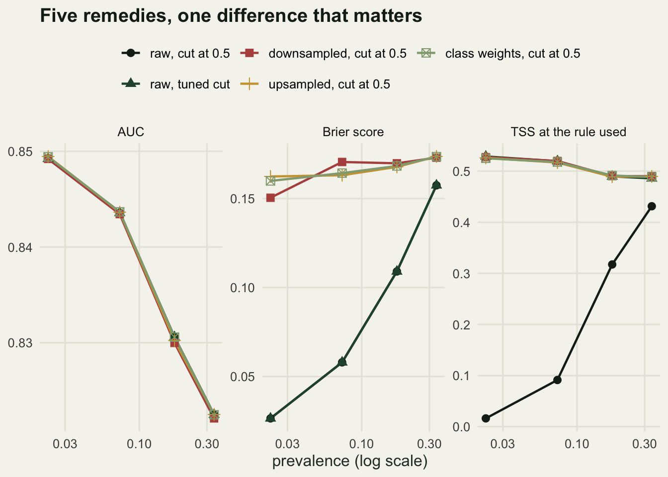

AUC, Brier score and true skill statistic at the operating rule for five treatments across four prevalences. Discrimination is flat, the Brier score punishes every resampled fit, and the true skill statistic separates only the raw model at 0.5 from everything else.

There is a detail in the top row of the table that I did not expect and that survives repetition. At prevalence 0.3365, where nobody would call the data imbalanced, the raw model at 0.5 scores 0.4313 while the best available score on the same ranking is 0.4899. The default threshold is not optimal even when the classes are nearly balanced. It is optimal when you want to minimise the raw error count and the two kinds of error cost the same, which is a decision problem no ecologist has ever actually had.

Upsampling and class weighting deserve one more look, because they are not two methods.

set.seed(2236)
tr_one <- sim_sites(n_train)
ip <- which(tr_one$occ == 1); iq <- which(tr_one$occ == 0)
m_raw <- glm(occ ~ elev + wet, data = tr_one, family = binomial)
up_rows <- c(iq, sample(ip, length(iq), replace = TRUE))
m_up <- glm(occ ~ elev + wet, data = tr_one[up_rows, ], family = binomial)
wgt <- ifelse(tr_one$occ == 1, length(iq) / length(ip), 1)
m_wt <- suppressWarnings(
  glm(occ ~ elev + wet, data = tr_one, family = binomial, weights = wgt))
print(round(rbind(raw = coef(m_raw), upsampled = coef(m_up), weighted = coef(m_wt)), 4))

          (Intercept)   elev     wet
raw           -4.4739 1.2202 -1.0177
upsampled     -1.1336 1.3519 -1.1439
weighted      -1.1022 1.3249 -1.1235

cat(sprintf("weight ratio %.2f, log of it %.4f, intercept shift of the weighted fit %.4f\n",
            length(iq) / length(ip), log(length(iq) / length(ip)),
            coef(m_wt)[1] - coef(m_raw)[1]))

weight ratio 32.06, log of it 3.4675, intercept shift of the weighted fit 3.3718

Upsampling with replacement to a weight ratio of 32.06 gives an intercept of -1.1336 and slopes of 1.3519 and -1.1439. Setting the weights directly gives -1.1022, 1.3249 and -1.1235. They are the same estimator: duplicating a row is exactly the same as multiplying its contribution to the log-likelihood, and the small gaps are the noise the resampling adds by drawing which presences to duplicate. The weighted intercept sits 3.3718 above the raw one, against a log weight ratio of 3.4675: the same offset, one more time, from a method that never mentions sampling fractions. The suppressed warning in that fit is glm objecting to non-integer weights on a binomial response, which is a warning about the standard errors, not about the point estimates.

Where a small presence count really does bite

None of this means the presence count is harmless. It means the harm is not in the ratio. Here is a regime where 12 presences ruin an estimate outright. Add a rare habitat type to the survey, a seepage patch, present at 12 of the 4000 sites and occupied with probability 0.85 when it occurs. Fit the model with the seep indicator included, over 400 replicate datasets.

set.seed(2645)
n_seep <- 12
p_seep <- 0.85
sim_seep <- function() {
  d <- sim_sites(n_train)
  d$seep <- 0
  d$seep[sample.int(n_train, n_seep)] <- 1
  d$occ[d$seep == 1] <- rbinom(n_seep, 1, p_seep)
  d
}
n_draw <- 400
sep_out <- as.data.frame(t(replicate(n_draw, {
  d <- sim_seep()
  fit <- suppressWarnings(glm(occ ~ elev + wet + seep, data = d, family = binomial))
  sc <- summary(fit)$coefficients
  c(occupied_seeps = sum(d$occ[d$seep == 1]), est = sc["seep", "Estimate"],
    se = sc["seep", "Std. Error"])
})))
cat(sprintf("%d datasets, %d seep sites each, true occupancy at a seep %.2f\n",
            n_draw, n_seep, p_seep))

400 datasets, 12 seep sites each, true occupancy at a seep 0.85

print(table(sep_out$occupied_seeps))

  6   7   8   9  10  11  12 
  1  10  26  63 121 115  64 

cat(sprintf("all %d seeps occupied in %.4f of datasets\n",
            n_seep, mean(sep_out$occupied_seeps == n_seep)))

all 12 seeps occupied in 0.1600 of datasets

for (kk in c(n_seep, n_seep - 1, n_seep - 2)) {
  sub_out <- sep_out[sep_out$occupied_seeps == kk, ]
  cat(sprintf("%d of %d seeps occupied (%d datasets): median estimate %.2f, median se %.2f\n",
              kk, n_seep, nrow(sub_out), median(sub_out$est), median(sub_out$se)))
}

12 of 12 seeps occupied (64 datasets): median estimate 21.99, median se 604.60
11 of 12 seeps occupied (115 datasets): median estimate 7.82, median se 1.16
10 of 12 seeps occupied (121 datasets): median estimate 6.80, median se 0.89

cat(sprintf("true seep contrast at an average site: %.4f\n", qlogis(p_seep) - b_int))

true seep contrast at an average site: 6.3346

In 0.16 of the datasets every seep was occupied, and in those 64 datasets the maximum likelihood estimate does not exist. R returns a number anyway: the median estimate is 21.99 with a median standard error of 604.60. Where one seep happened to be empty, the same coefficient is estimated at 7.82 with a standard error of 1.16, and where two were empty, 6.80 with 0.89, against a true contrast of 6.3346 at an average site. One absence is the difference between a usable estimate and a runaway one.

set.seed(9781)
repeat {
  seep_dat <- sim_seep()
  if (sum(seep_dat$occ[seep_dat$seep == 1]) == n_seep) break
}
fit_sep <- suppressWarnings(glm(occ ~ elev + wet + seep, data = seep_dat, family = binomial))
print(round(summary(fit_sep)$coefficients, 3))

            Estimate Std. Error z value Pr(>|z|)
(Intercept)   -4.584      0.177 -25.837    0.000
elev           1.276      0.114  11.214    0.000
wet           -0.957      0.107  -8.946    0.000
seep          21.927    654.544   0.033    0.973

seep_fix <- seep_dat
seep_fix$occ[which(seep_fix$seep == 1)[1]] <- 0
fit_fix <- suppressWarnings(glm(occ ~ elev + wet + seep, data = seep_fix, family = binomial))
print(round(summary(fit_fix)$coefficients, 3))

            Estimate Std. Error z value Pr(>|z|)
(Intercept)   -4.567      0.176 -25.962        0
elev           1.266      0.113  11.190        0
wet           -0.946      0.106  -8.890        0
seep           7.768      1.112   6.985        0

cat(sprintf("one absence added: estimate falls from %.2f to %.2f, se from %.1f to %.2f\n",
            coef(fit_sep)["seep"], coef(fit_fix)["seep"],
            summary(fit_sep)$coefficients["seep", "Std. Error"],
            summary(fit_fix)$coefficients["seep", "Std. Error"]))

one absence added: estimate falls from 21.93 to 7.77, se from 654.5 to 1.11

Look at what the summary table does with the separated fit. The seep coefficient is 21.927 with a standard error of 654.544, a z value of 0.033 and a p value of 0.973. The strongest predictor in the model, the one variable that perfectly determines the outcome wherever it occurs, is reported as the least significant term in the table. Flip a single one of those 12 seeps to absent and the estimate becomes 7.768 with a standard error of 1.112. The glm warning about fitted probabilities numerically 0 or 1, which the code above suppresses so that this comparison stays readable, is the diagnostic; it should never be ignored.

This is a small-sample problem and it has a small-sample fix. Penalised likelihood or a weakly informative prior on the coefficients pulls the estimate back to something finite without pretending to know more than the data say. That is worked through in Bayesian logistic regression under separation. Resampling the classes does not help here at all, and downsampling makes it worse by throwing away the absences that might have broken the separation.

What this cannot tell you

Everything above assumes two things that a real dataset rarely gives you. The model is correctly specified: the fitted equation is the one that generated the data, so there is no missing predictor, no wrong functional form, no spatial dependence. And the absences are real absences, recorded by someone who looked and did not find the species.

The second assumption is the one that collapses in most species distribution work. If your data are presence records plus background points sampled from a region, an “absence” is a point that may well hold the species. The consequence is not a bias to be corrected; it is that the intercept is not estimable from the sample at all, because you chose the number of background points yourself. Watch what that does.

set.seed(1123)
region <- sim_sites(400000)
occupied <- which(region$occ == 1)
use_pts <- sample(occupied, 600)
cat(sprintf("region %d cells, prevalence %.4f, presence records used %d\n",
            nrow(region), mean(region$occ), length(use_pts)))

region 400000 cells, prevalence 0.0288, presence records used 600

bg_grid <- c(2000, 5000, 20000)
bg_tab <- do.call(rbind, lapply(bg_grid, function(nb) {
  bg <- sample.int(nrow(region), nb)
  dd <- rbind(data.frame(region[use_pts, c("elev", "wet")], y_pb = 1),
              data.frame(region[bg, c("elev", "wet")], y_pb = 0))
  fit <- glm(y_pb ~ elev + wet, data = dd, family = binomial)
  data.frame(background = nb, occupied_background = sum(region$occ[bg]),
             intercept = unname(coef(fit)[1]), elev = unname(coef(fit)[2]),
             wet = unname(coef(fit)[3]))
}))
print(round(bg_tab, 4), row.names = FALSE)

 background occupied_background intercept   elev     wet
       2000                  61   -2.1113 1.1003 -0.7631
       5000                 161   -3.0781 1.1519 -0.8208
      20000                 560   -4.3781 1.0631 -0.7782

cat(sprintf("intercept moves %.4f then %.4f; log background ratios %.4f and %.4f\n",
            bg_tab$intercept[2] - bg_tab$intercept[1],
            bg_tab$intercept[3] - bg_tab$intercept[2],
            log(bg_grid[2] / bg_grid[1]), log(bg_grid[3] / bg_grid[2])))

intercept moves -0.9668 then -1.3000; log background ratios 0.9163 and 1.3863

cat(sprintf("elevation slope %.4f to %.4f against a true %.1f\n",
            min(bg_tab$elev), max(bg_tab$elev), b_elev))

elevation slope 1.0631 to 1.1519 against a true 1.3

The same 600 presence records, the same region, three analysts who chose 2000, 5000 and 20000 background points. The intercepts are -2.1113, -3.0781 and -4.3781. The moves between them are -0.9668 and -1.3000 against log background ratios of 0.9163 and 1.3863: the case-control offset again, except that this time there is no true intercept to correct back to, because the sampling fraction of a background point is an arbitrary decision and not a property of the landscape. Absolute occupancy probability is simply not in the data.

The slopes are still informative, which is why presence-background models work at all for ranking sites, but they are not clean either. Across the three fits the elevation slope runs between 1.0631 and 1.1519 against a true 1.3, attenuated because 61, 161 and 560 of the background points were themselves occupied, and calling an occupied cell a zero pulls the contrast towards nothing. That bias does not shrink as you add background points. It is a different problem from imbalance, it wears the same arithmetic, and no amount of resampling touches it.

Where to go next

The measurement that keeps recurring here is that the ranking survives everything and the probabilities do not. The next tutorial in this cluster takes that seriously: it works through what calibration means for a predicted probability of occurrence, how to measure it without the model refitting itself into agreement, and what to do about a model whose ranking you trust and whose numbers you do not.

References

King G, Zeng L 2001 Political Analysis 9(2):137-163 (10.1093/oxfordjournals.pan.a004868)

Allouche O, Tsoar A, Kadmon R 2006 Journal of Applied Ecology 43(6):1223-1232 (10.1111/j.1365-2664.2006.01214.x)

van den Goorbergh R, van Smeden M, Timmerman D, Van Calster B 2022 Journal of the American Medical Informatics Association 29(9):1525-1534 (10.1093/jamia/ocac093)

Guillera-Arroita G, Lahoz-Monfort JJ, Elith J, Gordon A, Kujala H, Lentini PE, McCarthy MA, Tingley R, Wintle BA 2015 Global Ecology and Biogeography 24(3):276-292 (10.1111/geb.12268)

Gelman A, Jakulin A, Pittau MG, Su YS 2008 Annals of Applied Statistics 2(4):1360-1383 (10.1214/08-AOAS191)

Related tutorials

• Calibrating predicted probabilities in R
• Data leakage in ecological model validation
• Choosing a decision threshold from costs
• Logistic regression for presence-absence data