library(ggplot2)

te_pal <- list(forest = "#275139", green = "#2f8f63", sage = "#93a87f",
               clay = "#b5534e", gold = "#cda23f", line = "#dad9ca",
               ink = "#16241d", paper = "#f5f4ee")

theme_te <- function() {
  theme_minimal(base_size = 12) +
    theme(panel.grid.minor = element_blank(),
          panel.grid.major = element_line(colour = "#e7e6dc"),
          plot.background = element_rect(fill = "#f5f4ee", colour = NA),
          panel.background = element_rect(fill = "#f5f4ee", colour = NA),
          plot.title = element_text(face = "bold", colour = te_pal$ink),
          axis.title = element_text(colour = "#2c3a31"))
}Choosing a decision threshold from costs
R
machine learning
model evaluation
conservation
ecology tutorial
ggplot2
Choosing a decision threshold in R: the cost ratio hidden in every ecological cut-off, decision curves and net benefit, and the price of miscalibration.
A distribution model hands a manager a number between 0 and 1 for every site. Nobody can act on a number between 0 and 1. You send the survey team or you do not, you buy the parcel or you do not, and somewhere between the prediction and the action a line gets drawn. That line is usually drawn without comment: 0.5 because it is the middle of the scale, or the cut that maximises the true skill statistic because a well-cited paper did that, or the observed prevalence because it looks like the species is being taken into account.
Each of those lines is a statement about the relative cost of two mistakes, whether or not anyone said so. Acting where the species is absent wastes a visit; not acting where it is present loses an occurrence. A threshold is the exchange rate between the two, and the common defaults set it silently, sometimes at a value the manager would reject on sight if it were written down.
This tutorial derives the threshold that minimises expected cost, checks it against a brute-force sweep on simulated held-out data, and reads the popular rules backwards to recover the cost ratio each one assumes. It then measures whether the model beats the trivial policies of acting everywhere and acting nowhere, what miscalibrated probabilities cost when the cost rule is applied to them, and how far the answer moves when the threshold is estimated from a survey. Everything is simulated in base R, with ggplot2 for the figures. If the upstream question is what a presence-absence model does when presences are scarce to begin with, that is Class imbalance in species presence models.
The threshold a cost ratio implies
Write cost_fp for the cost of acting at a site where the species turns out to be absent, and cost_fn for the cost of not acting at a site where it turns out to be present. At a site with probability p of presence, acting has expected cost cost_fp * (1 - p) and not acting has expected cost cost_fn * p. Acting is the cheaper choice exactly when cost_fp * (1 - p) < cost_fn * p, which rearranges to p > cost_fp / (cost_fp + cost_fn). Rearrange it once more, to p / (1 - p) > cost_fp / cost_fn, and the same rule reads: act when the odds of presence exceed the ratio of the cost of a wasted action to the cost of a missed occurrence.
Two consequences fall out of that one line of algebra. Only the ratio of the costs matters, so a manager who cannot price a survey visit in pounds can still use the rule if they can say a missed occurrence is worth four visits. And prevalence appears nowhere in it: rarity enters through p at each site, not through the threshold, so any rule that moves the cut when the species becomes rarer is doing something the cost calculation never asked for.
The test bed is a logistic model with two covariates, fitted to a training sample and applied to a large held-out set. The fitted model has the same form as the generating one, so its predictions are calibrated to within sampling error, which is what makes the formula applicable at all.
set.seed(20260815)
n_train <- 4000
n_pop <- 200000
beta0 <- -1.15
beta1 <- 1.20
beta2 <- -0.75

sim_sites <- function(nn, intercept) {
  x1 <- rnorm(nn)
  x2 <- rnorm(nn)
  pp <- plogis(intercept + beta1 * x1 + beta2 * x2)
  data.frame(y = rbinom(nn, 1, pp), x1 = x1, x2 = x2)
}

train_dat <- sim_sites(n_train, beta0)
pop_dat <- sim_sites(n_pop, beta0)
fit_main <- glm(y ~ x1 + x2, family = binomial, data = train_dat)
pop_dat$phat <- as.numeric(predict(fit_main, newdata = pop_dat, type = "response"))

auc_rank <- function(ph, yy) {
  rk <- rank(ph)
  n1 <- as.numeric(sum(yy == 1))
  n0 <- as.numeric(sum(yy == 0))
  (sum(rk[yy == 1]) - n1 * (n1 + 1) / 2) / (n1 * n0)
}

cat(sprintf("training sites %d, held-out sites %d\n", n_train, n_pop))
training sites 4000, held-out sites 200000cat(sprintf("prevalence: training %.4f, held-out %.4f\n",
mean(train_dat$y), mean(pop_dat$y)))prevalence: training 0.2913, held-out 0.3007cat(sprintf("held-out AUC %.4f\n", auc_rank(pop_dat$phat, pop_dat$y)))held-out AUC 0.8050cat(sprintf("mean predicted probability %.4f against observed %.4f\n",
mean(pop_dat$phat), mean(pop_dat$y)))mean predicted probability 0.2947 against observed 0.3007Prevalence is 0.3007 in the held-out set and 0.2913 in the training sample, the held-out AUC is 0.8050, and the mean predicted probability of 0.2947 sits close to the observed 0.3007. That last comparison is the weakest calibration check there is, but it has to pass before any of the arithmetic below means anything.
Sweeping a threshold is counting a confusion matrix once per candidate cut. Brute force over a fine grid on 200000 sites is wasteful, so the counts come from a single sort: order the predictions, take cumulative sums of the labels, and read off with findInterval how many presences and absences fall below any cut. One direct count checks the result, which is the cheapest way to catch an off-by-one in the interval convention.
sweep_counts <- function(ph, yy, thr_at) {
  o <- order(ph)
  ps <- ph[o]
  ys <- yy[o]
  n1 <- sum(ys)
  n0 <- length(ys) - n1
  k <- findInterval(thr_at, ps, left.open = TRUE)
  false_neg <- c(0, cumsum(ys))[k + 1]
  true_neg <- c(0, cumsum(1 - ys))[k + 1]
  data.frame(thr = thr_at, tp = n1 - false_neg, fp = n0 - true_neg,
             fn = false_neg, tn = true_neg)
}

thr_seq <- seq(0.001, 0.999, by = 0.001)
cnt_main <- sweep_counts(pop_dat$phat, pop_dat$y, thr_seq)

at_grid <- function(thr_at, target) which.min(abs(thr_at - target))
chk_at <- 0.37
chk_j <- at_grid(thr_seq, chk_at)
acted <- pop_dat$phat >= chk_at
cat(sprintf("thresholds on the grid: %d, from %.3f to %.3f\n",
            length(thr_seq), min(thr_seq), max(thr_seq)))
thresholds on the grid: 999, from 0.001 to 0.999cat(sprintf("cross-check at %.2f: sweep gives tp %d and fp %d, direct count %d and %d\n",
chk_at, cnt_main$tp[chk_j], cnt_main$fp[chk_j],
sum(acted & pop_dat$y == 1), sum(acted & pop_dat$y == 0)))cross-check at 0.37: sweep gives tp 37715 and fp 26449, direct count 37715 and 26449Both counts agree at 37715 true positives and 26449 false positives. Now put the formula on trial with three cost ratios: equal costs, a missed occurrence worth four wasted visits, and a threatened species where a missed occurrence is worth nineteen. For each, the analytic threshold is set against the one that actually minimises measured cost over 999 candidate cuts.
cost_curve <- function(cnt, cost_fp, cost_fn, nn) {
  (cost_fp * cnt$fp + cost_fn * cnt$fn) / nn
}

ratio_set <- c(1, 4, 19)
verify_tab <- do.call(rbind, lapply(ratio_set, function(rr) {
  cost_fp <- 1
  cost_fn <- rr
  t_star <- cost_fp / (cost_fp + cost_fn)
  cc <- cost_curve(cnt_main, cost_fp, cost_fn, n_pop)
  j <- which.min(cc)
  data.frame(cost_ratio = rr, analytic = t_star, empirical = thr_seq[j],
             cost_analytic = cc[which.min(abs(thr_seq - t_star))],
             cost_empirical = cc[j])
}))
verify_tab$excess <- verify_tab$cost_analytic - verify_tab$cost_empirical
print(round(verify_tab, 5))
cost_ratio analytic empirical cost_analytic cost_empirical excess
1 1 0.50 0.483 0.22986 0.22942 0.00043
2 4 0.20 0.197 0.47850 0.47793 0.00057
3 19 0.05 0.052 0.65563 0.65479 0.00084The analytic thresholds are 0.50, 0.20 and 0.05, and the empirical minima are 0.483, 0.197 and 0.052. The formula is right, and the residual disagreement is what a finite sample buys: the cost at the analytic threshold exceeds the cost at the empirical minimum by 0.00043, 0.00057 and 0.00084 per site, on costs of 0.22986, 0.47850 and 0.65563. The empirical winner wins by well under one per cent of the cost, and only because it was allowed to look at the data it is scored on.
The asymmetric case is the one to hold on to. With a missed occurrence priced at nineteen wasted visits the cost-optimal cut is 0.05: act at every site the model gives a one in twenty chance of holding the species. That is not a lax threshold, it is the arithmetic of the stated costs, and any manager who says a missed record of a threatened species is much worse than a fruitless visit has already agreed to something close to it.
panel_lab <- sprintf("cost ratio %d to 1", ratio_set)
cost_dat <- do.call(rbind, lapply(seq_along(ratio_set), function(i) {
  focus <- verify_tab$analytic[i]
  keep <- thr_seq >= focus / 4 & thr_seq <= min(0.9, focus * 4)
  data.frame(panel = panel_lab[i], thr = thr_seq[keep],
             cost = cost_curve(cnt_main, 1, ratio_set[i], n_pop)[keep])
}))
cost_dat$panel <- factor(cost_dat$panel, levels = panel_lab)
mark_dat <- data.frame(panel = factor(panel_lab, levels = panel_lab),
                       thr = verify_tab$empirical, cost = verify_tab$cost_empirical,
                       vline = verify_tab$analytic)

ggplot(cost_dat, aes(thr, cost)) +
  geom_line(colour = te_pal$forest, linewidth = 0.9) +
  geom_vline(data = mark_dat, aes(xintercept = vline),
             linetype = "dashed", colour = te_pal$clay) +
  geom_point(data = mark_dat, colour = te_pal$clay, size = 2.6) +
  facet_wrap(~ panel, scales = "free") +
  labs(title = "The formula lands where the data does",
       x = "decision threshold", y = "expected cost per site") +
  theme_te()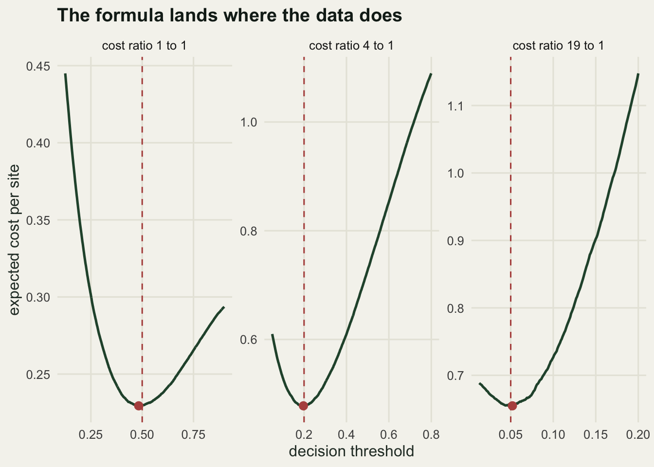
What the usual defaults are worth in costs
The formula runs backwards as easily as forwards. A threshold t is cost-optimal for exactly one ratio, cost_fn / cost_fp = (1 - t) / t, so any rule that produces a number between 0 and 1 has an opinion about costs and can be asked to state it. Four rules are tested here: the fixed 0.5, the cut that maximises the true skill statistic, the cut that equalises sensitivity and specificity, and the cut set at the observed prevalence.
They are applied twice, to two settings that differ only in the intercept of the generating model. In the first the species occupies about three sites in ten; in the second it is scarce. The covariate coefficients, and therefore the ecology the model can see, are identical.
set.seed(20260816)
beta0_rare <- -3.30
train_rare <- sim_sites(n_train, beta0_rare)
pop_rare <- sim_sites(n_pop, beta0_rare)
fit_rare <- glm(y ~ x1 + x2, family = binomial, data = train_rare)
pop_rare$phat <- as.numeric(predict(fit_rare, newdata = pop_rare, type = "response"))

rules_for <- function(ph, yy) {
  cnt <- sweep_counts(ph, yy, thr_seq)
  sens <- cnt$tp / (cnt$tp + cnt$fn)
  spec <- cnt$tn / (cnt$tn + cnt$fp)
  thr_rule <- c(0.5, thr_seq[which.max(sens + spec - 1)],
                thr_seq[which.min(abs(sens - spec))], round(mean(yy), 3))
  data.frame(threshold = thr_rule, implied_ratio = (1 - thr_rule) / thr_rule)
}

rule_name <- c("fixed 0.5", "max TSS", "sens = spec", "prevalence")
common_rules <- rules_for(pop_dat$phat, pop_dat$y)
rare_rules <- rules_for(pop_rare$phat, pop_rare$y)
implied_tab <- data.frame(rule = rule_name,
                          thr_common = common_rules$threshold,
                          ratio_common = common_rules$implied_ratio,
                          thr_rare = rare_rules$threshold,
                          ratio_rare = rare_rules$implied_ratio)
cat(sprintf("common setting: prevalence %.4f, AUC %.4f\n",
            mean(pop_dat$y), auc_rank(pop_dat$phat, pop_dat$y)))
common setting: prevalence 0.3007, AUC 0.8050cat(sprintf("rare setting: prevalence %.4f, AUC %.4f\n",
mean(pop_rare$y), auc_rank(pop_rare$phat, pop_rare$y)))rare setting: prevalence 0.0728, AUC 0.8219print(format(implied_tab, digits = 3)) rule thr_common ratio_common thr_rare ratio_rare
1 fixed 0.5 0.500 1.00 0.500 1.0
2 max TSS 0.287 2.48 0.077 12.0
3 sens = spec 0.297 2.37 0.078 11.8
4 prevalence 0.301 2.32 0.073 12.7cat(sprintf("max TSS implied ratio moves by a factor of %.2f\n",
implied_tab$ratio_rare[2] / implied_tab$ratio_common[2]))max TSS implied ratio moves by a factor of 4.83The fixed cut of 0.5 implies a cost ratio of 1.00 in both settings, which is at least honest about being arbitrary: it says a wasted visit and a missed occurrence are worth the same, everywhere, for every species. Almost nobody believes that, and it is stated in almost every paper that uses the default.
The other three rules are the interesting ones. At prevalence 0.3007 they put the cut at 0.287, 0.297 and 0.301, implying cost ratios of 2.48, 2.37 and 2.32. At prevalence 0.0728 they put it at 0.077, 0.078 and 0.073, implying 12.0, 11.8 and 12.7. The three land in the same place in both settings, and the place is set by the prevalence: for a calibrated model, maximising the true skill statistic puts the cut where the slope of the ROC curve is 1, which for a calibrated probability is where the threshold equals the prevalence. The implied ratio is then just the odds of absence, (1 - prevalence) / prevalence. What looks like three different pieces of methodology is one rule wearing three hats.
The consequence deserves saying slowly. The manager’s costs did not change between the two settings. Nothing about the survey budget, the value of a record, or the conservation status moved. Only the species got rarer, and the max-TSS rule quietly multiplied the implied cost ratio by 4.83. Sometimes that is defensible: a rarer species may genuinely be worth more per occurrence. But then it is a judgement about value, and it should be made by the person who owns the budget, with a number they recognise, rather than arriving as a side effect of an optimisation criterion that was chosen because it is the one the methods papers use.
Net benefit and the decision curve
Knowing the cost-optimal threshold does not tell you whether to use the model at all. The manager always has two policies that need no model: act everywhere, and act nowhere. Net benefit is the standard way of putting all three on one axis. At threshold t it is TP / n - (FP / n) * t / (1 - t), that is, true positives per site with false positives charged at the exchange rate the threshold implies.
The units are worth unpicking, because net benefit looks arbitrary until you connect it back to the cost calculation. Expected cost per site is (cost_fp * FP + cost_fn * FN) / n, and since false negatives are the presences you did not act on, that equals cost_fn * (prevalence - net benefit). Maximising net benefit and minimising expected cost are the same operation, viewed at different scales. Net benefit just quotes the answer in units of occurrences found per site, which is a currency a manager can hold.
net_benefit <- function(ph, yy, thr_at) {
  cnt <- sweep_counts(ph, yy, thr_at)
  nn <- length(yy)
  cnt$tp / nn - (cnt$fp / nn) * thr_at / (1 - thr_at)
}
nb_treat_all <- function(prev, thr_at) prev - (1 - prev) * thr_at / (1 - thr_at)

nb_seq <- seq(0.02, 0.60, by = 0.005)
nb_model <- net_benefit(pop_dat$phat, pop_dat$y, nb_seq)
nb_all <- nb_treat_all(mean(pop_dat$y), nb_seq)
wins <- nb_model > nb_all & nb_model > 0
cat(sprintf("thresholds examined %d, from %.2f to %.2f\n",
            length(nb_seq), min(nb_seq), max(nb_seq)))
thresholds examined 117, from 0.02 to 0.60cat(sprintf("calibrated model beats both defaults at %d of them, from %.2f to %.2f\n",
sum(wins), min(nb_seq[wins]), max(nb_seq[wins])))calibrated model beats both defaults at 117 of them, from 0.02 to 0.60j20 <- at_grid(nb_seq, 0.20)
cat(sprintf("at threshold %.2f: model %.4f, treat all %.4f, treat none %.4f\n",
nb_seq[j20], nb_model[j20], nb_all[j20], 0))at threshold 0.20: model 0.1810, treat all 0.1258, treat none 0.0000The calibrated model beats both defaults at all 117 thresholds on the grid, from 0.02 to 0.60. At a threshold of 0.20 it returns 0.1810 against 0.1258 for acting everywhere and 0.0000 for acting nowhere. That clean sweep is not luck and it is not evidence that the model is good. It is a property of calibration: if the predicted probability is the true one, then every site the rule acts on has p at least t, so its contribution to net benefit, p - (1 - p) * t / (1 - t), cannot be negative, and the sites the rule skips are exactly the ones that would have dragged the treat-all policy down. A calibrated model cannot lose a decision curve comparison. Anything that does lose one has a calibration problem, not a discrimination problem.
So here is a failure, built on purpose. Take the same fitted model, with no change to its coefficients, and apply it in a region where the species is much commoner than where it was trained. This is the ordinary life of a distribution model: fitted in one catchment, borrowed for the next. Discrimination survives the move almost intact, because the covariates still rank sites correctly. The probabilities do not.
set.seed(20260817)
beta0_hi <- 0.30
pop_hi <- sim_sites(n_pop, beta0_hi)
pop_hi$phat <- as.numeric(predict(fit_main, newdata = pop_hi, type = "response"))

nb_hi <- net_benefit(pop_hi$phat, pop_hi$y, nb_seq)
nb_hi_all <- nb_treat_all(mean(pop_hi$y), nb_seq)
mgr_lo <- 0.05
mgr_hi <- 0.25
in_mgr <- nb_seq >= mgr_lo & nb_seq <= mgr_hi
cat(sprintf("transfer region: prevalence %.4f, AUC %.4f, mean predicted %.4f\n",
            mean(pop_hi$y), auc_rank(pop_hi$phat, pop_hi$y), mean(pop_hi$phat)))
transfer region: prevalence 0.5540, AUC 0.8029, mean predicted 0.2963cat(sprintf("manager range %.2f to %.2f: model beats treat all at %d of %d thresholds\n",
mgr_lo, mgr_hi, sum(nb_hi[in_mgr] > nb_hi_all[in_mgr]), sum(in_mgr)))manager range 0.05 to 0.25: model beats treat all at 0 of 41 thresholdsj10 <- at_grid(nb_seq, 0.10)
cat(sprintf("at threshold %.2f: model %.4f, treat all %.4f, shortfall %.4f\n",
nb_seq[j10], nb_hi[j10], nb_hi_all[j10], nb_hi_all[j10] - nb_hi[j10]))at threshold 0.10: model 0.4800, treat all 0.5044, shortfall 0.0244cat(sprintf("the transferred model overtakes treat all only above %.3f\n",
min(nb_seq[nb_hi > nb_hi_all])))the transferred model overtakes treat all only above 0.450In the new region the species occupies 0.5540 of sites and the model predicts a mean of 0.2963. Its AUC is 0.8029, which any reviewer would accept, and it is worse than doing nothing clever at all: over the whole band a manager who fears missing an occurrence would work in, thresholds from 0.05 to 0.25, the model beats acting everywhere at 0 of 41 thresholds. At 0.10 the model returns 0.4800 against 0.5044 for acting everywhere, a shortfall of 0.0244 occurrences per site. It only overtakes the trivial policy above 0.450, a threshold that implies a missed occurrence is worth slightly more than a wasted visit, which is far weaker than what the manager said.
The construction is deliberate and the ingredients are stated: respectable ranking, badly displaced probabilities, and a decision region at low thresholds where acting everywhere is cheap because the species is common. What makes it worth building is that none of the summaries usually reported would catch it. AUC is fine. The ROC curve is fine. The sensitivity and specificity at the chosen cut are fine. The decision curve is the only one of these that asks whether the model earns its place against a policy that requires no model.
nb_panel <- c("calibrated, own region", "transferred, commoner region")
nb_dat <- rbind(
  data.frame(panel = nb_panel[1], thr = nb_seq, nb = nb_model, kind = "model"),
  data.frame(panel = nb_panel[1], thr = nb_seq, nb = nb_all, kind = "treat all"),
  data.frame(panel = nb_panel[1], thr = nb_seq, nb = 0, kind = "treat none"),
  data.frame(panel = nb_panel[2], thr = nb_seq, nb = nb_hi, kind = "model"),
  data.frame(panel = nb_panel[2], thr = nb_seq, nb = nb_hi_all, kind = "treat all"),
  data.frame(panel = nb_panel[2], thr = nb_seq, nb = 0, kind = "treat none"))
nb_dat$panel <- factor(nb_dat$panel, levels = nb_panel)
band_dat <- data.frame(panel = factor(nb_panel, levels = nb_panel),
                       x1 = mgr_lo, x2 = mgr_hi)

ggplot(nb_dat, aes(thr, nb, colour = kind, linetype = kind)) +
  geom_rect(data = band_dat, aes(xmin = x1, xmax = x2, ymin = -Inf, ymax = Inf),
            inherit.aes = FALSE, fill = te_pal$sage, alpha = 0.22) +
  geom_line(linewidth = 0.9) +
  facet_wrap(~ panel) +
  scale_colour_manual(values = c(te_pal$forest, te_pal$clay, te_pal$ink)) +
  scale_linetype_manual(values = c("solid", "solid", "dashed")) +
  coord_cartesian(ylim = c(-0.1, 0.6)) +
  labs(title = "Beating treat all is not automatic",
       x = "decision threshold", y = "net benefit per site",
       colour = NULL, linetype = NULL) +
  theme_te() +
  theme(legend.position = "top")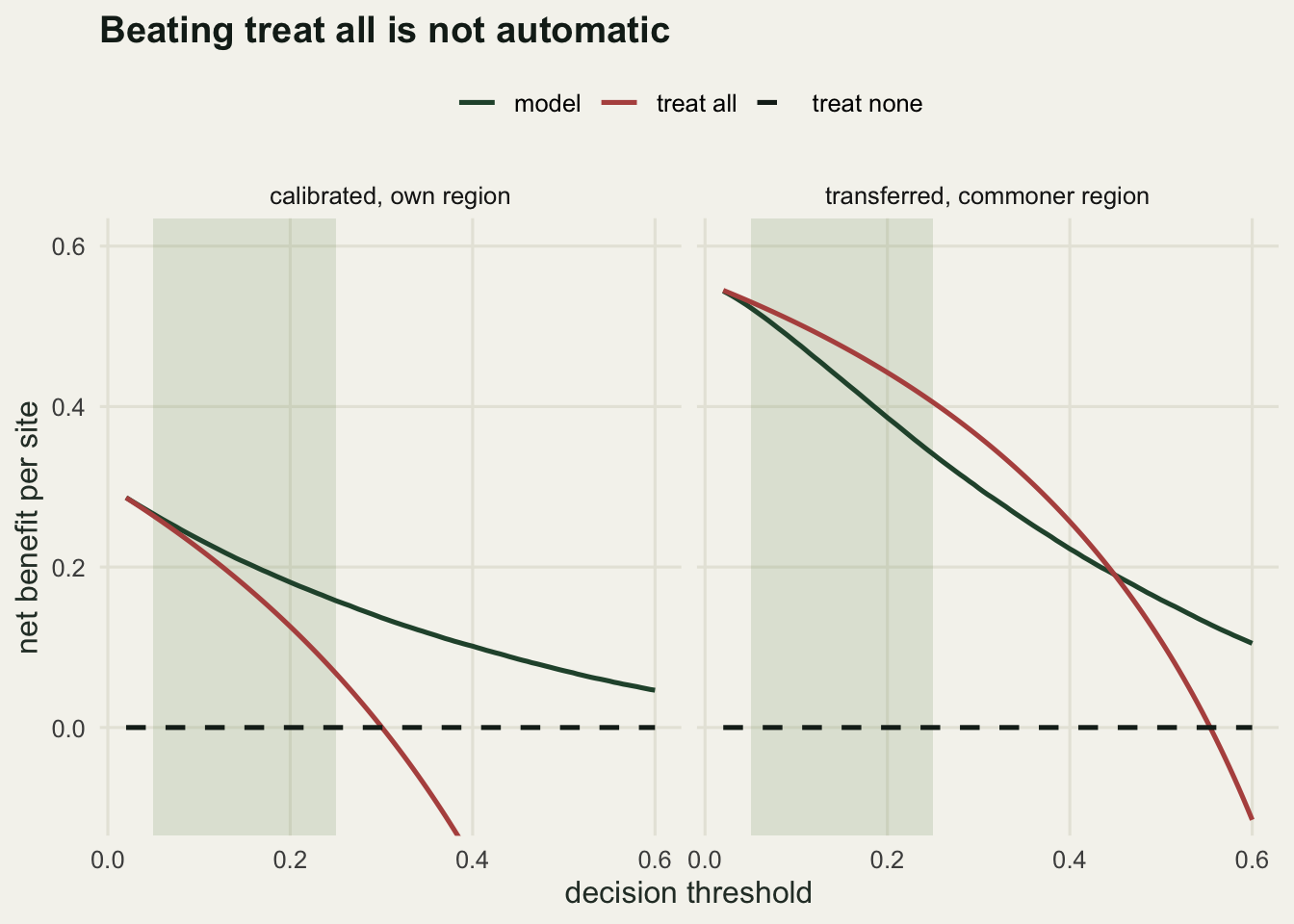
What miscalibration costs at a fixed AUC
The threshold rule is a statement about probabilities, so it is only as good as the probabilities. Discrimination is invariant to any monotone rescaling of the predictions: squash them, stretch them, run them through any increasing function and the AUC is unchanged, because the ranking is unchanged. The cost-optimal threshold is not invariant to anything of the sort, because it names an actual value on the probability scale.
To price that, take the calibrated predictions and push them through plogis(2 * qlogis(p)), which doubles the logit and so drives predictions towards 0 and 1. This is the signature of an overfitted model: too confident, in both directions, while ranking sites perfectly well. Half the held-out data is set aside for recalibration and the other half for evaluation, and the cost rule for the four to one ratio is applied to all three versions of the predictions.
set.seed(20260818)
half_i <- sample.int(n_pop, n_pop / 2)
cal_dat <- pop_dat[half_i, ]
eval_dat <- pop_dat[-half_i, ]

distort <- function(ph) plogis(2 * qlogis(ph))
cal_dat$p_dist <- distort(cal_dat$phat)
eval_dat$p_dist <- distort(eval_dat$phat)

fit_cal <- glm(y ~ qlogis(p_dist), family = binomial, data = cal_dat)
eval_dat$p_recal <- as.numeric(predict(fit_cal, newdata = eval_dat, type = "response"))

cost_fp <- 1
cost_fn <- 4
t_star <- cost_fp / (cost_fp + cost_fn)
realised_cost <- function(ph, yy, thr) {
  act <- ph >= thr
  (cost_fp * sum(act & yy == 0) + cost_fn * sum(!act & yy == 1)) / length(yy)
}

cat(sprintf("calibration sites %d, evaluation sites %d, cost ratio %d to 1, t* %.2f\n",
            nrow(cal_dat), nrow(eval_dat), cost_fn / cost_fp, t_star))
calibration sites 100000, evaluation sites 100000, cost ratio 4 to 1, t* 0.20cat(sprintf("AUC calibrated %.4f, distorted %.4f, recalibrated %.4f\n",
auc_rank(eval_dat$phat, eval_dat$y), auc_rank(eval_dat$p_dist, eval_dat$y),
auc_rank(eval_dat$p_recal, eval_dat$y)))AUC calibrated 0.8065, distorted 0.8065, recalibrated 0.8065cat(sprintf("mean predicted: calibrated %.4f, distorted %.4f, recalibrated %.4f, observed %.4f\n",
mean(eval_dat$phat), mean(eval_dat$p_dist), mean(eval_dat$p_recal),
mean(eval_dat$y)))mean predicted: calibrated 0.2942, distorted 0.2364, recalibrated 0.3000, observed 0.3003cost_good <- realised_cost(eval_dat$phat, eval_dat$y, t_star)
cost_bad <- realised_cost(eval_dat$p_dist, eval_dat$y, t_star)
cost_fix <- realised_cost(eval_dat$p_recal, eval_dat$y, t_star)
cat(sprintf("cost per site at t*: calibrated %.4f, distorted %.4f, recalibrated %.4f\n",
cost_good, cost_bad, cost_fix))cost per site at t*: calibrated 0.4772, distorted 0.5448, recalibrated 0.4773cat(sprintf("excess from miscalibration alone %.4f, that is %.1f percent\n",
cost_bad - cost_good, 100 * (cost_bad - cost_good) / cost_good))excess from miscalibration alone 0.0676, that is 14.2 percentcat(sprintf("recovered by recalibration %.4f\n", cost_bad - cost_fix))recovered by recalibration 0.0675cc_dist <- cost_curve(sweep_counts(eval_dat$p_dist, eval_dat$y, thr_seq),
cost_fp, cost_fn, nrow(eval_dat))
cat(sprintf("on the distorted scale the best cut is %.3f, giving cost %.4f\n",
thr_seq[which.min(cc_dist)], min(cc_dist)))on the distorted scale the best cut is 0.057, giving cost 0.4769cat(sprintf("the distorted image of t* is %.4f\n", distort(t_star)))the distorted image of t* is 0.0588cat(sprintf("cutting the distorted scale at t* really cuts the true scale at %.4f\n",
plogis(qlogis(t_star) / 2)))cutting the distorted scale at t* really cuts the true scale at 0.3333All three versions have an AUC of 0.8065 to four decimals, because the distortion and the recalibration are both monotone. Applying the same cost-optimal threshold of 0.20 to each, the cost per site is 0.4772 for the calibrated predictions and 0.5448 for the distorted ones: an excess of 0.0676 per site, 14.2 per cent, caused by nothing except the shape of the map from evidence to probability. Recalibrating on the held-out half and applying the same rule recovers 0.0675 of that 0.0676, landing at 0.4773.
The mechanism is visible in one number. Cutting the distorted scale at 0.20 means acting only where the true probability is at least 0.3333, because that is where the doubled logit crosses the cut. The manager asked for a threshold of 0.20 and got 0.3333, so the model skips a band of sites that were worth acting on at four to one, and each skipped occurrence is charged at four.
There is an honest qualification, and it goes the other way. The ranking was never damaged, so a threshold tuned directly on the distorted scale finds a cut of 0.057 with a cost of 0.4769, which matches the calibrated result. Miscalibration does not destroy the information in the model. It breaks the interpretation of the threshold, which is the one thing the cost formula depends on. Calibration is what makes the formula usable; the machinery for checking and fixing it is in Calibrating predicted probabilities in R.
rel_bins <- function(ph, yy, tag, n_bin = 20) {
  br <- unique(quantile(ph, seq(0, 1, length.out = n_bin + 1)))
  g <- cut(ph, br, include.lowest = TRUE)
  data.frame(kind = tag, pred = as.numeric(tapply(ph, g, mean)),
             obs = as.numeric(tapply(yy, g, mean)))
}
rel_dat <- rbind(rel_bins(eval_dat$phat, eval_dat$y, "calibrated"),
                 rel_bins(eval_dat$p_dist, eval_dat$y, "distorted"),
                 rel_bins(eval_dat$p_recal, eval_dat$y, "recalibrated"))

ggplot(rel_dat, aes(pred, obs, colour = kind, shape = kind)) +
  geom_abline(slope = 1, intercept = 0, colour = te_pal$sage, linewidth = 1.1) +
  geom_vline(xintercept = t_star, linetype = "dashed", colour = te_pal$ink) +
  geom_point(size = 2.4) +
  geom_line(linewidth = 0.6) +
  scale_colour_manual(values = c(te_pal$forest, te_pal$clay, te_pal$gold)) +
  labs(title = "Same ranking, different probabilities",
       x = "mean predicted probability in bin", y = "observed frequency in bin",
       colour = NULL, shape = NULL) +
  theme_te() +
  theme(legend.position = "top")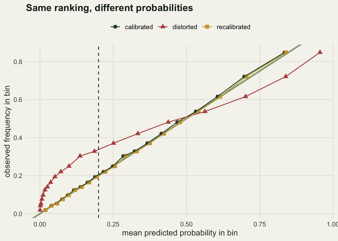
How exactly does the threshold have to be right
Everything so far treated the threshold as known. It is known when it comes from a cost ratio, and estimated when it comes from data, and the data-driven rules of the second section are all estimates from a finite sample. A survey of 500 sites is a generous real dataset. Bootstrap the max-TSS threshold on one.
set.seed(20260819)
n_small <- 500
n_boot <- 1000
survey <- eval_dat[sample.int(nrow(eval_dat), n_small), ]

tss_thr <- function(ph, yy) {
  cnt <- sweep_counts(ph, yy, thr_seq)
  tss <- cnt$tp / (cnt$tp + cnt$fn) + cnt$tn / (cnt$tn + cnt$fp) - 1
  thr_seq[which.max(tss)]
}
boot_thr <- replicate(n_boot, {
  ii <- sample.int(n_small, n_small, replace = TRUE)
  tss_thr(survey$phat[ii], survey$y[ii])
})
qq <- unname(quantile(boot_thr, c(0.025, 0.975)))
cat(sprintf("survey sites %d with %d presences, bootstrap resamples %d\n",
            n_small, sum(survey$y), n_boot))
survey sites 500 with 154 presences, bootstrap resamples 1000cat(sprintf("max TSS threshold on the survey %.3f, bootstrap mean %.3f, sd %.3f\n",
tss_thr(survey$phat, survey$y), mean(boot_thr), sd(boot_thr)))max TSS threshold on the survey 0.340, bootstrap mean 0.305, sd 0.068cat(sprintf("bootstrap 2.5 to 97.5 percent interval %.3f to %.3f, width %.3f\n",
qq[1], qq[2], qq[2] - qq[1]))bootstrap 2.5 to 97.5 percent interval 0.175 to 0.431, width 0.256cat(sprintf("implied cost ratio at those ends: %.1f to 1 and %.1f to 1\n",
(1 - qq[1]) / qq[1], (1 - qq[2]) / qq[2]))implied cost ratio at those ends: 4.7 to 1 and 1.3 to 1The survey of 500 sites holds 154 presences and gives a max-TSS threshold of 0.340. Over 1000 bootstrap resamples the same rule ranges from 0.175 to 0.431 at the 2.5 and 97.5 per cent points, a width of 0.256, with a standard deviation of 0.068. A quarter of the probability scale, from a rule that gets quoted to three decimal places in methods sections. The implied cost ratio at the two ends of that interval is roughly 4.7 to 1 at one end and 1.3 to 1 at the other, which are different management policies.
Estimation noise in the threshold is not the same thing as cost, though, and the second quantity is the one that matters. Draw 400 independent surveys of 500 sites, pick the cost-minimising cut on each by brute force, and score that cut against the full evaluation set.
set.seed(20260820)
n_rep <- 400
est_thr <- replicate(n_rep, {
  ii <- sample.int(nrow(eval_dat), n_small)
  cc <- cost_curve(sweep_counts(eval_dat$phat[ii], eval_dat$y[ii], thr_seq),
                   cost_fp, cost_fn, n_small)
  thr_seq[which.min(cc)]
})
cost_of <- function(thr) realised_cost(eval_dat$phat, eval_dat$y, thr)
cost_est <- vapply(est_thr, cost_of, numeric(1))
cat(sprintf("replicate surveys %d of %d sites each\n", n_rep, n_small))
replicate surveys 400 of 500 sites eachcat(sprintf("estimated cut: mean %.3f, sd %.3f, against the formula value %.2f\n",
mean(est_thr), sd(est_thr), t_star))estimated cut: mean 0.203, sd 0.047, against the formula value 0.20cat(sprintf("cost with the estimated cut %.4f, with the formula %.4f\n",
mean(cost_est), cost_of(t_star)))cost with the estimated cut 0.4869, with the formula 0.4772cat(sprintf("penalty for estimating rather than computing %.4f, that is %.2f percent\n",
mean(cost_est) - cost_of(t_star),
100 * (mean(cost_est) - cost_of(t_star)) / cost_of(t_star)))penalty for estimating rather than computing 0.0097, that is 2.04 percentThe estimated cut averages 0.203 with a standard deviation of 0.047, so it is aimed at the right place and wanders around it. The cost of using it is 0.4869 against 0.4772 for the formula: a penalty of 0.0097 per site, 2.04 per cent, for estimating something that was available in closed form. Small, and it stays small precisely because the cost curve near its minimum is nearly flat, which is the same reason the empirical minima in the first section were only better by a fraction of a per cent.
That flatness has to be taken seriously in both directions. If misplacing the threshold by 0.047 costs 2 per cent, then getting the cost ratio slightly wrong cannot be expensive either, and a long argument about whether the ratio is 4 or 5 is not worth having. The sweep below assumes a ratio, sets the threshold from it, and scores the result against the true costs.
excess_for <- function(true_ratio) {
  assumed <- exp(seq(log(1), log(60), length.out = 121))
  cnt_a <- sweep_counts(eval_dat$phat, eval_dat$y, 1 / (1 + assumed))
  cc <- cost_curve(cnt_a, 1, true_ratio, nrow(eval_dat))
  best <- min(cost_curve(sweep_counts(eval_dat$phat, eval_dat$y, thr_seq),
                         1, true_ratio, nrow(eval_dat)))
  data.frame(true_ratio = sprintf("true ratio %d to 1", true_ratio),
             assumed = assumed, excess = cc / best - 1)
}
flat_dat <- rbind(excess_for(4), excess_for(19))
report_at <- c(1, 2, 4, 8, 19, 40)
for (rr in report_at) {
  a4 <- flat_dat[flat_dat$true_ratio == "true ratio 4 to 1", ]
  a19 <- flat_dat[flat_dat$true_ratio == "true ratio 19 to 1", ]
  cat(sprintf("assumed ratio %5.1f: excess %.3f when the truth is 4, %.3f when it is 19\n",
              rr, a4$excess[which.min(abs(a4$assumed - rr))],
              a19$excess[which.min(abs(a19$assumed - rr))]))
}
assumed ratio 1.0: excess 0.517 when the truth is 4, 3.870 when it is 19
assumed ratio 2.0: excess 0.147 when the truth is 4, 2.062 when it is 19
assumed ratio 4.0: excess 0.000 when the truth is 4, 0.731 when it is 19
assumed ratio 8.0: excess 0.083 when the truth is 4, 0.151 when it is 19
assumed ratio 19.0: excess 0.279 when the truth is 4, 0.002 when it is 19
assumed ratio 40.0: excess 0.394 when the truth is 4, 0.025 when it is 19tol <- 0.05
for (tag in unique(flat_dat$true_ratio)) {
sub_dat <- flat_dat[flat_dat$true_ratio == tag & flat_dat$excess < tol, ]
cat(sprintf("%s: within %.2f of optimal for assumed ratios %.1f to %.1f\n",
tag, tol, min(sub_dat$assumed), max(sub_dat$assumed)))
}true ratio 4 to 1: within 0.05 of optimal for assumed ratios 2.7 to 6.5
true ratio 19 to 1: within 0.05 of optimal for assumed ratios 11.3 to 60.0When the true ratio is four to one, assuming anything between 2.7 and 6.5 keeps the cost within 5 per cent of the best available. When it is nineteen to one, the tolerant window runs from 11.3 to beyond the end of the sweep. Precision in the ratio is not what this exercise is for.
The other end of the range is a different story. Assuming equal costs when the truth is four to one, which is exactly what the 0.5 default does, costs an excess of 0.517: half as much again as the optimal policy. When the truth is nineteen to one the same default costs an excess of 3.870, so the bill is almost five times what it needed to be. Getting the order of magnitude right matters a great deal; getting the second digit right does not matter at all. The valley is also asymmetric, and in the useful direction: at a true ratio of four, assuming eight costs 0.083 while assuming two costs 0.147, so erring towards caution is cheaper than erring towards complacency.
ratio_lab <- c("true ratio 4 to 1", "true ratio 19 to 1")
truth_dat <- data.frame(true_ratio = factor(ratio_lab, levels = ratio_lab),
                        vline = c(4, 19))
flat_dat$true_ratio <- factor(flat_dat$true_ratio, levels = ratio_lab)

ggplot(flat_dat, aes(assumed, excess, colour = true_ratio)) +
  geom_hline(yintercept = tol, colour = te_pal$ink, linetype = "dotted",
             linewidth = 0.7) +
  geom_vline(data = truth_dat, aes(xintercept = vline, colour = true_ratio),
             linetype = "dashed", show.legend = FALSE) +
  geom_line(linewidth = 0.9) +
  scale_colour_manual(values = c(te_pal$forest, te_pal$clay)) +
  scale_x_log10(breaks = c(1, 2, 5, 10, 20, 50)) +
  coord_cartesian(ylim = c(0, 1)) +
  labs(title = "A shallow valley, not a spike",
       x = "assumed cost ratio", y = "relative excess cost", colour = NULL) +
  theme_te() +
  theme(legend.position = "top")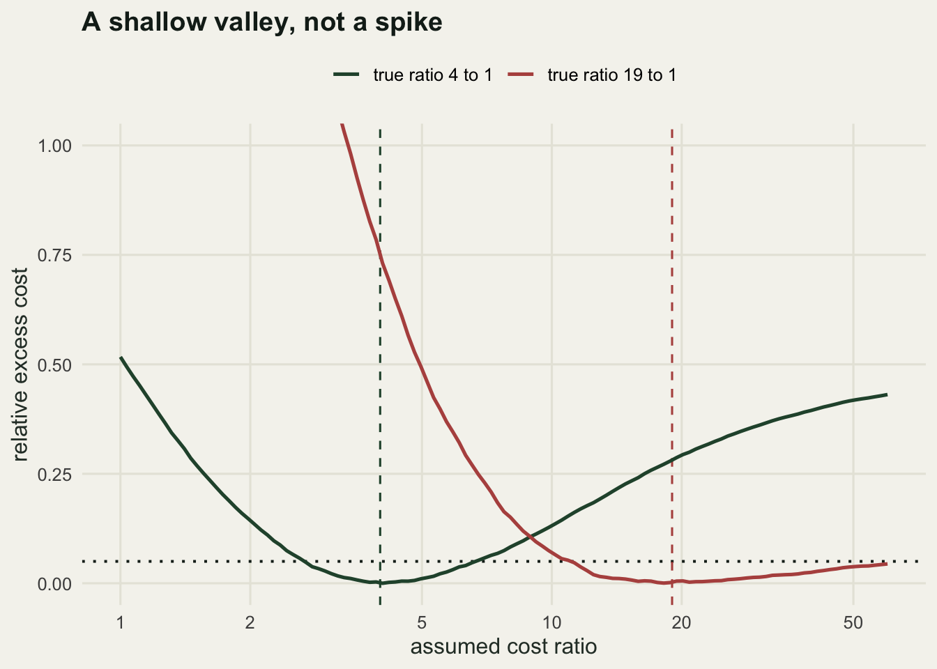
What a cost ratio cannot capture
The whole framework rests on one assumption that conservation rarely satisfies: that the two errors are measured in the same units. A wasted survey visit costs staff days and fuel. A missed occurrence costs a population, or a legal obligation, or the credibility of the next recommendation. Setting the ratio to nineteen is not a measurement, it is an exchange rate imposed between things that do not trade, and no amount of arithmetic downstream makes it one.
The two errors also usually land on different people. The wasted visit is paid by the survey team, the missed occurrence by the species and by whoever inherits the site in ten years. A single cost ratio expresses the preferences of whoever chose it, and the choice is a political act dressed as a parameter. That is not an argument against writing it down. It is an argument for writing it down where others can see it, which is more than a bare 0.5 achieves.
Then there is the additivity built into the arithmetic. Expected cost sums the cost of each error independently, so the tenth wasted visit costs exactly what the first one did. Under a fixed budget it does not: the tenth visit may be the one that exhausts the season, and its real cost is the survey that never happened. The same applies at the other end, where a missed occurrence matters more if it is the last population than if it is one of forty. A decision-theoretic treatment of a budget constraint is a different piece of machinery, usually a knapsack problem, and the threshold rule is not it.
Nothing above tests whether the model’s probability refers to the quantity the decision cares about, either. A distribution model predicts suitability or occupancy at the time of sampling. The manager acts next year, over a site that may have burned, dried out or been grazed. The threshold rule is exact with respect to a probability that may be answering an adjacent question. The value of the exercise is the argument it forces: someone has to say out loud how much worse a missed occurrence is than a wasted visit. The number that comes out the other side is not precise, and the flat cost surface says it does not have to be.
Where to go next
This closes a run of four tutorials on the hygiene of a predictive model. The leakage post ends with a validation estimate you can believe; the class imbalance post ends with a model that has not been wrecked by rarity and a set of metrics that survive it; the calibration post ends with probabilities that mean what they say. This one spends all three: an honest probability, on an honest held-out set, converted into an action by a threshold somebody chose on purpose. Take any of the three away and the threshold rule quietly stops being valid.
Two sideways steps from here. The evaluation of distribution models has its own conventions, and the question of which summary answers which decision is worked through in the species distribution model evaluation tutorial. And the same logic runs inside a detection pipeline, where the score is a recogniser confidence rather than a probability of occupancy and the errors are false clips against missed calls: Score thresholds and precision in bioacoustics does that case, including what happens to the arithmetic when the prevalence of real calls collapses.
References
Vickers AJ, Elkin EB 2006 Medical Decision Making 26(6):565-574 (10.1177/0272989X06295361)
Liu C, Berry PM, Dawson TP, Pearson RG 2005 Ecography 28(3):385-393 (10.1111/j.0906-7590.2005.03957.x)
Allouche O, Tsoar A, Kadmon R 2006 Journal of Applied Ecology 43(6):1223-1232 (10.1111/j.1365-2664.2006.01214.x)
Guillera-Arroita G, Lahoz-Monfort JJ, Elith J, Gordon A, Kujala H, Lentini PE, McCarthy MA, Tingley R, Wintle BA 2015 Global Ecology and Biogeography 24(3):276-292 (10.1111/geb.12268)
Van Calster B, Wynants L, Verbeek JFM, Verbakel JY, Christodoulou E, Vickers AJ, Roobol MJ, Steyerberg EW 2018 European Urology 74(6):796-804 (10.1016/j.eururo.2018.08.038)