Score thresholds and precision in bioacoustics

Choosing a score threshold for an acoustic recogniser in R: why AUC ignores prevalence, why precision collapses at a quiet site, and how to validate clips.

A species recogniser does not hand you detections. It hands you candidate detections, each with a confidence score, and leaves you to decide where to cut. Above the cut you keep the clip and treat it as a record of the species; below it you throw the clip away. Every number that comes out of the survey afterwards, an occupancy estimate or an activity index, inherits whatever mixture of real calls and rain, wind and other species sits above that line. Choosing the line is the analysis, not a preliminary to it.

The usual way of reporting how well a recogniser performs is the area under the ROC curve. It is the wrong summary for this decision, and it is wrong in a specific way: AUC is a statement about ranks, computed within the true calls and within the false ones separately, and it does not know how many of each you have. Precision does know. This tutorial takes one recogniser with one fixed pair of score distributions, moves only the prevalence of real calls, and shows that AUC does not move at all while precision falls by a factor of nearly five at the same threshold. Then it shows what that does to the threshold you should be using, and what it does to the validation effort you spend listening to clips.

Everything below is simulated, so the truth is known and the arithmetic can be checked against it. If you want the upstream half of this, how a table of scored detections should be treated as data in the first place, that is in Automated acoustic detections as data.

library(ggplot2)

te_pal <- list(forest = "#275139", green = "#2f8f63", sage = "#93a87f",
               clay = "#b5534e", gold = "#cda23f", line = "#dad9ca",
               ink = "#16241d", paper = "#f5f4ee")

theme_te <- function() {
  theme_minimal(base_size = 12) +
    theme(panel.grid.minor = element_blank(),
          panel.grid.major = element_line(colour = "#e7e6dc"),
          plot.background = element_rect(fill = "#f5f4ee", colour = NA),
          panel.background = element_rect(fill = "#f5f4ee", colour = NA),
          plot.title = element_text(face = "bold", colour = te_pal$ink),
          axis.title = element_text(colour = "#2c3a31"))
}

One recogniser, two sites

The recogniser is a pair of beta distributions on the score. True calls are drawn from Beta(4, 3) and false candidates from Beta(2, 5). The two distributions overlap heavily, which is what a real recogniser looks like once you are past the easy loud calls. Nothing about those two distributions changes anywhere in this post. The only thing that changes is the prevalence: the fraction of candidate detections that are real. The rich site is a wetland edge where 0.40 of the candidates are the target species; the poor site is a dry plot at the range margin where 0.02 of them are.

set.seed(20260814)
a_sig <- 4; b_sig <- 3
a_noi <- 2; b_noi <- 5
n_cand <- 300000
prev_rich <- 0.40
prev_poor <- 0.02

sim_site <- function(n, prev) {
  yy <- rbinom(n, 1, prev)
  score <- ifelse(yy == 1, rbeta(n, a_sig, b_sig), rbeta(n, a_noi, b_noi))
  data.frame(y = yy, sc = score)
}

site_rich <- sim_site(n_cand, prev_rich)
site_poor <- sim_site(n_cand, prev_poor)

cat(sprintf("candidates per site: %d\n", n_cand))

candidates per site: 300000

cat(sprintf("prevalence rich %.2f, poor %.2f\n", prev_rich, prev_poor))

prevalence rich 0.40, poor 0.02

cat(sprintf("mean score, true calls %.3f; false calls %.3f\n",
            a_sig / (a_sig + b_sig), a_noi / (a_noi + b_noi)))

mean score, true calls 0.571; false calls 0.286

cat(sprintf("true detections in the two pools: %d and %d\n",
            sum(site_rich$y), sum(site_poor$y)))

true detections in the two pools: 120002 and 6004

Mean score 0.571 for a true call against 0.286 for a false one, with both distributions spread across the whole interval. The picture is the one every bioacoustician recognises: the modes are well apart, the tails are not.

xg <- seq(0.002, 0.998, length.out = 400)
dens_dat <- data.frame(
  score = rep(xg, 2),
  dens = c(dbeta(xg, a_noi, b_noi), dbeta(xg, a_sig, b_sig)),
  kind = rep(c("false candidate", "true call"), each = length(xg)))

ggplot(dens_dat, aes(score, dens, colour = kind, fill = kind)) +
  geom_area(alpha = 0.25, position = "identity", linewidth = 0.9) +
  geom_vline(xintercept = 0.60, linetype = "dashed", colour = te_pal$ink) +
  scale_colour_manual(values = c(te_pal$clay, te_pal$forest)) +
  scale_fill_manual(values = c(te_pal$clay, te_pal$forest)) +
  labs(title = "The recogniser, before any threshold",
       x = "recogniser score", y = "density", colour = NULL, fill = NULL) +
  theme_te() +
  theme(legend.position = "top")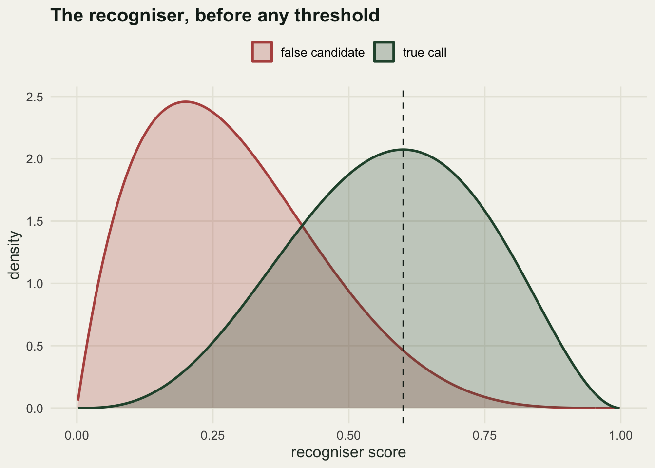

Score distributions for true and false candidate detections. These two curves are fixed throughout the post; only the mixing weight between them changes.

The confusion matrix, counted by hand

Fix a working threshold of 0.60 and count the four cells directly. There is no package here: above is a logical vector, and the four counts are sums of logical conjunctions. Precision is the fraction of kept clips that are real, recall is the fraction of real calls that are kept, specificity is the fraction of false candidates correctly dropped, and F1 is the harmonic mean of precision and recall.

thr_work <- 0.60

count_conf <- function(d, thr) {
  above <- d$sc >= thr
  c(tp = sum(above & d$y == 1), fp = sum(above & d$y == 0),
    fn = sum(!above & d$y == 1), tn = sum(!above & d$y == 0))
}

metrics_from <- function(k) {
  prec <- unname(k["tp"] / (k["tp"] + k["fp"]))
  rec  <- unname(k["tp"] / (k["tp"] + k["fn"]))
  spec <- unname(k["tn"] / (k["tn"] + k["fp"]))
  c(precision = prec, recall = rec, specificity = spec,
    f1 = 2 * prec * rec / (prec + rec))
}

k_rich <- count_conf(site_rich, thr_work)
tab_rich <- matrix(c(k_rich["tp"], k_rich["fn"], k_rich["fp"], k_rich["tn"]),
                   nrow = 2,
                   dimnames = list(c("kept (score >= 0.60)", "dropped"),
                                   c("truth: call", "truth: noise")))
cat(sprintf("working threshold: %.2f\n", thr_work))

working threshold: 0.60

print(tab_rich)

                     truth: call truth: noise
kept (score >= 0.60)       54786         7346
dropped                    65216       172652

print(round(metrics_from(k_rich), 4))

  precision      recall specificity          f1 
     0.8818      0.4565      0.9592      0.6016 

At the rich site the threshold keeps 54786 real calls and 7346 false ones, so precision is 0.8818: of every hundred clips you keep, about eighty-eight are the species. Recall is 0.4565, meaning the threshold also throws away 65216 real calls, more than half of them. Specificity is 0.9592 and F1 is 0.6016. Specificity is the number to watch here, because it is the one that will mislead you in a moment: it is computed entirely within the false candidates, and 0.9592 sounds like a small error rate right up to the point where the false candidates outnumber the true ones fifty to one.

The same recogniser, and a precision that collapses

Now run the identical threshold at the poor site. AUC comes from the rank statistic: the Mann-Whitney form, the probability that a randomly chosen true call scores above a randomly chosen false one. Compute it from ranks and also analytically from the two beta densities, which is possible precisely because AUC is a functional of the two conditional score distributions and of nothing else.

auc_rank <- function(d) {
  rk <- rank(d$sc)
  n1 <- as.numeric(sum(d$y == 1))
  n0 <- as.numeric(sum(d$y == 0))
  (sum(rk[d$y == 1]) - n1 * (n1 + 1) / 2) / (n1 * n0)
}
auc_theory <- integrate(function(x) dbeta(x, a_sig, b_sig) * pbeta(x, a_noi, b_noi),
                        0, 1)$value

k_poor <- count_conf(site_poor, thr_work)
cat(sprintf("AUC  rich %.4f   poor %.4f   analytic %.4f\n",
            auc_rank(site_rich), auc_rank(site_poor), auc_theory))

AUC  rich 0.8794   poor 0.8793   analytic 0.8788

cat(sprintf("recall    rich %.4f   poor %.4f\n",
            metrics_from(k_rich)["recall"], metrics_from(k_poor)["recall"]))

recall    rich 0.4565   poor 0.4554

cat(sprintf("specificity rich %.4f poor %.4f\n",
            metrics_from(k_rich)["specificity"], metrics_from(k_poor)["specificity"]))

specificity rich 0.9592 poor 0.9593

cat(sprintf("precision rich %.4f   poor %.4f   ratio %.2f\n",
            metrics_from(k_rich)["precision"], metrics_from(k_poor)["precision"],
            metrics_from(k_rich)["precision"] / metrics_from(k_poor)["precision"]))

precision rich 0.8818   poor 0.1861   ratio 4.74

cat(sprintf("kept clips rich %d   poor %d\n",
            unname(k_rich["tp"] + k_rich["fp"]), unname(k_poor["tp"] + k_poor["fp"])))

kept clips rich 62132   poor 14688

AUC is 0.8794 at the rich site and 0.8793 at the poor one, against an analytic value of 0.8788; the difference between the two sites is simulation noise and nothing else. Recall agrees between the sites to within the same noise (0.4565 against 0.4554) and so does specificity (0.9592 against 0.9593), for the same reason: each is computed inside one of the two label classes. Precision is 0.8818 at the rich site and 0.1861 at the poor one, a ratio of 4.74. Four clips in five that you keep at the poor site are not the species.

Say that plainly, because it is the whole point. A recogniser validated on a rich dataset and deployed on a poor one has the same AUC, the same recall, the same specificity, and a precision the analyst never measured. The published performance figure survives the move; the thing you actually needed does not. And the absolute volume matters too: the poor site still hands you 14688 clips above the threshold, against 62132 at the rich site, so the false material does not even look thin.

ROC agrees where precision-recall does not

Both curves are built from the same sorted score vector. Sort the candidates by score descending, take cumulative sums of the labels, and every prefix of that vector is the set kept by one threshold. From the cumulative counts, the false positive rate and true positive rate give the ROC curve, and recall with precision gives the precision-recall curve. The areas come from the trapezium rule over the curve as drawn.

roc_pr <- function(d) {
  o <- order(-d$sc)
  yy <- d$y[o]
  tp <- cumsum(yy)
  fp <- cumsum(1 - yy)
  n1 <- sum(yy); n0 <- length(yy) - n1
  data.frame(cut_at = d$sc[o], fpr = fp / n0, tpr = tp / n1,
             recall = tp / n1, precision = tp / (tp + fp))
}
trap_area <- function(x, yv) sum(diff(x) * (head(yv, -1) + tail(yv, -1)) / 2)

cur_rich <- roc_pr(site_rich)
cur_poor <- roc_pr(site_poor)
auprc_rich <- trap_area(cur_rich$recall, cur_rich$precision)
auprc_poor <- trap_area(cur_poor$recall, cur_poor$precision)
cat(sprintf("ROC area   rich %.4f   poor %.4f\n",
            trap_area(cur_rich$fpr, cur_rich$tpr), trap_area(cur_poor$fpr, cur_poor$tpr)))

ROC area   rich 0.8794   poor 0.8793

cat(sprintf("PR area    rich %.4f   poor %.4f\n", auprc_rich, auprc_poor))

PR area    rich 0.8329   poor 0.2335

cat(sprintf("no-skill PR baseline  rich %.2f   poor %.2f\n", prev_rich, prev_poor))

no-skill PR baseline  rich 0.40   poor 0.02

cat(sprintf("PR area over baseline rich %.2f   poor %.2f\n",
            auprc_rich / prev_rich, auprc_poor / prev_poor))

PR area over baseline rich 2.08   poor 11.67

panel_lv <- c("ROC", "precision-recall")
thin_idx <- function(cur) unique(round(seq(50, nrow(cur), length.out = 900)))
one_frame <- function(cur, tag) {
  i <- thin_idx(cur)
  rbind(data.frame(panel = panel_lv[1], site = tag, x = cur$fpr[i], yv = cur$tpr[i]),
        data.frame(panel = panel_lv[2], site = tag,
                   x = cur$recall[i], yv = cur$precision[i]))
}
site_lv <- c("poor site, prevalence 0.02", "rich site, prevalence 0.40")
curve_dat <- rbind(one_frame(cur_poor, site_lv[1]), one_frame(cur_rich, site_lv[2]))
curve_dat$panel <- factor(curve_dat$panel, levels = panel_lv)
curve_dat$site <- factor(curve_dat$site, levels = site_lv)
base_dat <- data.frame(
  panel = factor(c(panel_lv[1], panel_lv[1], panel_lv[2], panel_lv[2],
                   panel_lv[2], panel_lv[2]), levels = panel_lv),
  x = c(0, 1, 0, 1, 0, 1),
  yv = c(0, 1, prev_rich, prev_rich, prev_poor, prev_poor),
  grp = c("a", "a", "b", "b", "d", "d"))

ggplot(curve_dat, aes(x, yv, colour = site, linewidth = site)) +
  geom_line(data = base_dat, aes(x, yv, group = grp), inherit.aes = FALSE,
            linetype = "dashed", linewidth = 0.5, colour = te_pal$ink) +
  geom_line(alpha = 0.85) +
  facet_wrap(~ panel) +
  scale_colour_manual(values = c(te_pal$clay, te_pal$forest)) +
  scale_linewidth_manual(values = c(2.4, 1), guide = "none") +
  coord_cartesian(xlim = c(0, 1), ylim = c(0, 1)) +
  labs(title = "Same ranks, different usefulness",
       x = "false positive rate (ROC) or recall (precision-recall)",
       y = "true positive rate or precision", colour = NULL) +
  theme_te() +
  theme(legend.position = "top")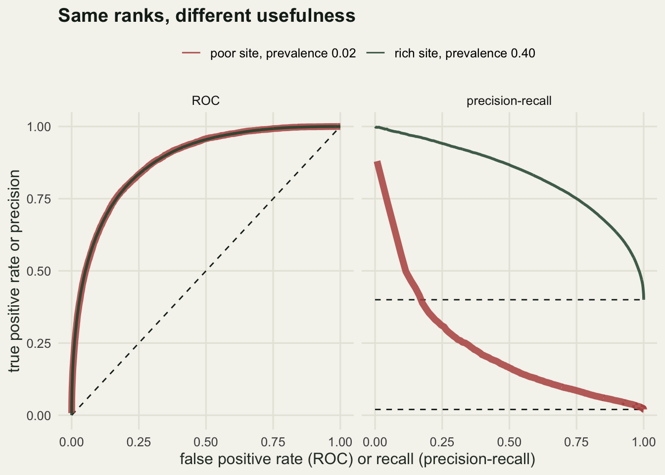

ROC and precision-recall curves for the same recogniser at two prevalences. The ROC curves lie on top of each other, so the poor site is drawn as a wide band with the rich site as a thin line inside it. The precision-recall curves separate completely. Dashed lines are the no-skill baselines.

The ROC areas are 0.8794 and 0.8793. The precision-recall areas are 0.8329 and 0.2335, against no-skill baselines of 0.40 and 0.02, since a coin flip that keeps a random subset of candidates has precision equal to the prevalence at every recall. This is the figure the post exists for: two panels, the same data, and only one of them changes when the ecology changes.

There is a trap in the fix, though, and it is worth measuring rather than glossing. If you report the precision-recall area as a multiple of its own baseline, the poor site scores 11.67 and the rich site only 2.08. Read that way the recogniser looks better at the poor site, which is nonsense from the point of view of anyone who has to listen to the clips. The area over baseline is a real quantity: it says the ranking is doing more work where the prevalence is low. It is simply not the quantity that tells you what fraction of your retained clips are the species. That number is 0.2335 at best, averaged across thresholds, and there is no summary statistic that rescues it.

The threshold that maximises F1 moves with the prevalence

If precision depends on prevalence and recall does not, then any criterion that balances the two must depend on prevalence as well. Sweep 91 thresholds across four simulated sites and find the F1 maximum at each.

prev_grid <- c(0.40, 0.20, 0.05, 0.02)
thr_grid <- seq(0.05, 0.95, by = 0.01)
cat(sprintf("thresholds swept: %d from %.2f to %.2f\n",
            length(thr_grid), min(thr_grid), max(thr_grid)))

thresholds swept: 91 from 0.05 to 0.95

sweep_f1 <- function(d) {
  vapply(thr_grid, function(tt) unname(metrics_from(count_conf(d, tt))["f1"]),
         numeric(1))
}
sites_all <- lapply(prev_grid, function(pv) sim_site(n_cand, pv))
f1_all <- lapply(sites_all, sweep_f1)

best_row <- function(i) {
  j <- which.max(f1_all[[i]])
  m <- metrics_from(count_conf(sites_all[[i]], thr_grid[j]))
  data.frame(prevalence = prev_grid[i], best_thr = thr_grid[j],
             f1 = unname(m["f1"]), precision = unname(m["precision"]),
             recall = unname(m["recall"]))
}
best_tab <- do.call(rbind, lapply(seq_along(prev_grid), best_row))
print(round(best_tab, 4))

  prevalence best_thr     f1 precision recall
1       0.40     0.41 0.7559    0.7104 0.8077
2       0.20     0.49 0.6279    0.5867 0.6754
3       0.05     0.60 0.4069    0.3678 0.4554
4       0.02     0.67 0.2932    0.2711 0.3193

The maximising threshold climbs from 0.41 at prevalence 0.40 to 0.67 at prevalence 0.02, and the F1 attained falls from 0.7559 to 0.2932. The direction is worth holding on to: the scarcer the species, the higher you have to cut, because each retained clip has to fight a larger pile of noise to earn its place.

f1_dat <- do.call(rbind, lapply(seq_along(prev_grid), function(i)
  data.frame(prevalence = factor(prev_grid[i], levels = prev_grid),
             thr = thr_grid, f1 = f1_all[[i]])))
pk_dat <- data.frame(prevalence = factor(best_tab$prevalence, levels = prev_grid),
                     thr = best_tab$best_thr, f1 = best_tab$f1)

ggplot(f1_dat, aes(thr, f1, colour = prevalence)) +
  geom_line(linewidth = 0.9) +
  geom_point(data = pk_dat, size = 2.6) +
  scale_colour_manual(values = c(te_pal$clay, te_pal$gold,
                                 te_pal$green, te_pal$forest)) +
  labs(title = "Where to cut depends on how common the species is",
       x = "score threshold", y = "F1", colour = "prevalence") +
  theme_te()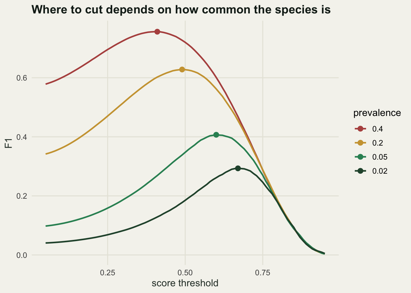

F1 against score threshold at four prevalences. Points mark the maximum of each curve; the maximum shifts to the right as the species becomes scarcer.

Carrying a threshold across sites is what happens in practice, because the threshold is usually chosen once, on the pilot data, and then written into the processing script.

thr_rich_best <- best_tab$best_thr[1]
poor_site <- sites_all[[4]]
carry <- metrics_from(count_conf(poor_site, thr_rich_best))
own <- metrics_from(count_conf(poor_site, best_tab$best_thr[4]))
cat(sprintf("carry threshold %.2f to the 0.02 site: precision %.4f, F1 %.4f\n",
            thr_rich_best, carry["precision"], carry["f1"]))

carry threshold 0.41 to the 0.02 site: precision 0.0699, F1 0.1285

cat(sprintf("its own best threshold %.2f gives: precision %.4f, F1 %.4f\n",
            best_tab$best_thr[4], own["precision"], own["f1"]))

its own best threshold 0.67 gives: precision 0.2711, F1 0.2932

cat(sprintf("loss: precision %.4f, F1 %.4f (F1 down %.1f percent)\n",
            own["precision"] - carry["precision"], own["f1"] - carry["f1"],
            100 * (own["f1"] - carry["f1"]) / own["f1"]))

loss: precision 0.2013, F1 0.1647 (F1 down 56.2 percent)

The rich site’s threshold of 0.41, applied at the poor site, gives precision 0.0699 and F1 0.1285. The poor site’s own threshold of 0.67 gives precision 0.2711 and F1 0.2932. That is 0.2013 of precision and 0.1647 of F1 given away, an F1 that is 56.2 percent lower than it needed to be, for a decision that was never revisited.

Validating a stratified subset without fooling yourself

None of the above is available in the field, because the labels are not. What you have is a listening budget. Take one million candidate clips from a season of recording at 0.02 prevalence, keep everything above 0.60, and ask what fraction of the retained set is real.

set.seed(20260815)
n_clip <- 1000000
prev_field <- 0.02
thr_keep <- 0.60
y_field <- rbinom(n_clip, 1, prev_field)
sc_field <- ifelse(y_field == 1, rbeta(n_clip, a_sig, b_sig), rbeta(n_clip, a_noi, b_noi))
kept <- sc_field >= thr_keep
y_kept <- y_field[kept]
sc_kept <- sc_field[kept]
n_kept <- length(y_kept)
prec_true <- mean(y_kept)
cat(sprintf("candidate clips %d, retained above %.2f: %d\n", n_clip, thr_keep, n_kept))

candidate clips 1000000, retained above 0.60: 49447

cat(sprintf("true precision of the retained set: %.4f (%d real calls)\n",
            prec_true, sum(y_kept)))

true precision of the retained set: 0.1820 (9001 real calls)

Nobody validates 49447 clips by drawing them at random, because at this precision most of the listening is spent confirming noise. The design people actually use is stratified: listen to every clip above some high score, where the yield is good, and to a thin random sample of the rest.

cut_hi <- 0.85
budget <- 3000
in_hi <- sc_kept >= cut_hi
n_hi <- sum(in_hi)
n_lo <- sum(!in_hi)
n_lo_draw <- budget - n_hi
cat(sprintf("listening budget %d clips\n", budget))

listening budget 3000 clips

cat(sprintf("high stratum (score >= %.2f): %d clips, all listened, precision %.4f\n",
            cut_hi, n_hi, mean(y_kept[in_hi])))

high stratum (score >= 0.85): 1335 clips, all listened, precision 0.7243

cat(sprintf("low stratum: %d clips, %d listened (1 in %.1f), precision %.4f\n",
            n_lo, n_lo_draw, n_lo / n_lo_draw, mean(y_kept[!in_hi])))

low stratum: 48112 clips, 1665 listened (1 in 28.9), precision 0.1670

cat(sprintf("high stratum share of the retained set: %.4f\n", n_hi / n_kept))

high stratum share of the retained set: 0.0270

A budget of 3000 clips covers all 1335 clips scoring above 0.85, where precision is 0.7243, and 1665 of the 48112 remaining clips, 1 in 28.9 of them, where precision is 0.1670. Now estimate the precision of the whole retained set two ways: by pooling the listened clips as though they were a simple random sample, and by weighting each listened clip by the inverse of its probability of having been selected.

lo_index <- which(!in_hi)
draw_once <- function() {
  picked <- sample(lo_index, n_lo_draw)
  y_lo <- y_kept[picked]
  y_hi <- y_kept[in_hi]
  naive <- (sum(y_hi) + sum(y_lo)) / budget
  wts <- c(rep(1, n_hi), rep(n_lo / n_lo_draw, n_lo_draw))
  yv <- c(y_hi, y_lo)
  c(naive = naive, weighted = sum(wts * yv) / sum(wts))
}
one <- draw_once()
cat(sprintf("one validation round: naive %.4f, weighted %.4f, truth %.4f\n",
            one["naive"], one["weighted"], prec_true))

one validation round: naive 0.4080, weighted 0.1697, truth 0.1820

n_rep <- 500
reps <- t(replicate(n_rep, draw_once()))
srs_est <- replicate(n_rep, mean(y_kept[sample.int(n_kept, budget)]))
est_tab <- data.frame(
  mean_est = c(mean(reps[, "naive"]), mean(reps[, "weighted"]), mean(srs_est)),
  bias = c(mean(reps[, "naive"]) - prec_true, mean(reps[, "weighted"]) - prec_true,
           mean(srs_est) - prec_true),
  se = c(sd(reps[, "naive"]), sd(reps[, "weighted"]), sd(srs_est)),
  row.names = c("naive pooled", "weighted", "simple random"))
cat(sprintf("replicates: %d, truth %.4f\n", n_rep, prec_true))

replicates: 500, truth 0.1820

print(round(est_tab, 4))

              mean_est   bias     se
naive pooled    0.4150 0.2330 0.0050
weighted        0.1820 0.0000 0.0087
simple random   0.1822 0.0001 0.0067

cat(sprintf("se ratio, weighted over simple random: %.3f\n",
            sd(reps[, "weighted"]) / sd(srs_est)))

se ratio, weighted over simple random: 1.297

The naive pooled estimate averages 0.4150 against a truth of 0.1820: a bias of 0.2330, more than twice the quantity being estimated. It is also the most stable of the three estimators, with a standard error of 0.0050, which is exactly what makes it dangerous. A tight confidence interval around the wrong number is the worst possible output of a validation exercise, and this is the number that gets quoted in a methods section as “precision was 41.5 percent based on 3000 validated clips”.

The weighted estimator recovers the truth: mean 0.1820, bias 0.0000 to four decimals. Its standard error is 0.0087.

est_dat <- data.frame(
  estimator = rep(c("naive pooled", "weighted", "simple random"), each = n_rep),
  value = c(reps[, "naive"], reps[, "weighted"], srs_est))

ggplot(est_dat, aes(value, colour = estimator, fill = estimator)) +
  geom_density(alpha = 0.25, linewidth = 0.9) +
  geom_vline(xintercept = prec_true, linetype = "dashed", colour = te_pal$ink) +
  scale_colour_manual(values = c(te_pal$clay, te_pal$gold, te_pal$forest)) +
  scale_fill_manual(values = c(te_pal$clay, te_pal$gold, te_pal$forest)) +
  labs(title = "Where the three estimators land",
       x = "estimated precision of the retained set", y = "density",
       colour = NULL, fill = NULL) +
  theme_te() +
  theme(legend.position = "top")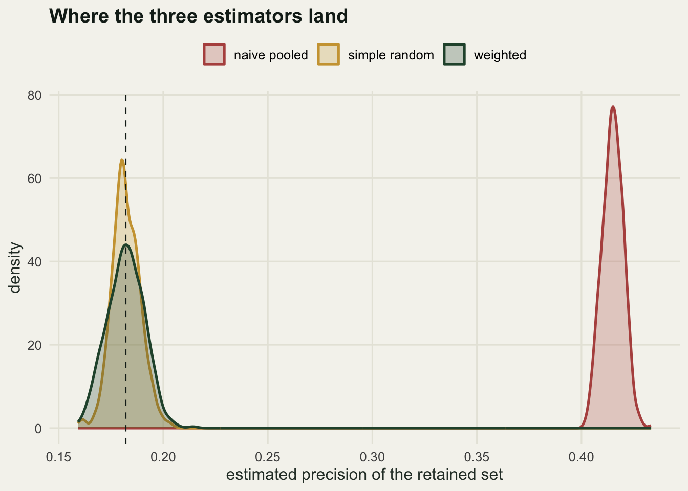

Sampling distributions of three precision estimators over 500 replicate validation rounds, with the true precision marked. The naive pooled estimator is tight and badly displaced.

Here is the part that did not come out the way the design story suggests. The simple random sample of the same 3000 clips has a standard error of 0.0067, smaller than the weighted estimator’s 0.0087, a ratio of 1.297. On these numbers the stratified design widens the interval rather than narrowing it. The reason is arithmetic: the high stratum is only 0.0270 of the retained set but eats 1335 of the 3000 listening slots, leaving the low stratum, which carries almost all of the weight, with a thinner sample than a plain random draw would have given it.

sd_strat <- function(nn) {
  nh <- round(n_hi / n_kept * nn)
  nl <- nn - nh
  nd <- budget - nh
  wl <- nl / nn
  p_lo <- mean(y_kept[!in_hi])
  sqrt(wl^2 * p_lo * (1 - p_lo) / nd * (1 - nd / nl))
}
sd_srs <- function(nn) sqrt((1 - budget / nn) * prec_true * (1 - prec_true) / budget)
size_grid <- c(5000, 10000, 20000, n_kept)
eff_tab <- data.frame(retained = size_grid,
                      sd_weighted = vapply(size_grid, sd_strat, numeric(1)),
                      sd_random = vapply(size_grid, sd_srs, numeric(1)))
eff_tab$ratio <- eff_tab$sd_weighted / eff_tab$sd_random
print(round(eff_tab, 5))

  retained sd_weighted sd_random   ratio
1     5000     0.00435   0.00446 0.97561
2    10000     0.00589   0.00589 0.99944
3    20000     0.00684   0.00650 1.05286
4    49447     0.00874   0.00683 1.27977

cross <- uniroot(function(nn) sd_strat(nn) - sd_srs(nn), c(4000, 40000))$root
cat(sprintf("break-even retained-set size: %.0f (budget covers %.2f of it)\n",
            cross, budget / cross))

break-even retained-set size: 10117 (budget covers 0.30 of it)

Holding the same budget and the same stratum proportions, and shrinking the retained set, the weighted estimator overtakes the simple random sample at about 10117 retained clips, which is where the budget covers 0.30 of the set. That is the regime the design belongs in: a small enough retained set that listening to the whole high stratum is a large fraction of the work, so the finite population correction does the job the stratification was supposed to. With a full season of one million clips behind it, it does not. What stratification does buy at any size is the high stratum itself, listened to exhaustively, which is the material most analyses actually keep; the mistake is to let that stratum’s labels stand in for the whole set.

The last piece is how much listening is enough. For a proportion, the standard error is the square root of p times one minus p over n, so pinning precision to plus or minus 0.05 needs the sample size below, checked against 20000 simulated validation rounds.

prec_targets <- c(0.50, 0.85)
half_width <- 0.05
z_crit <- 1.96
n_needed <- ceiling(z_crit^2 * prec_targets * (1 - prec_targets) / half_width^2)
cat(sprintf("half-width %.2f, z %.2f\n", half_width, z_crit))

half-width 0.05, z 1.96

for (i in seq_along(prec_targets)) {
  cover <- mean(abs(rbinom(20000, n_needed[i], prec_targets[i]) / n_needed[i] -
                      prec_targets[i]) <= half_width)
  cat(sprintf("true precision %.2f: need %d clips, simulated coverage %.4f\n",
              prec_targets[i], n_needed[i], cover))
}

true precision 0.50: need 385 clips, simulated coverage 0.9477
true precision 0.85: need 196 clips, simulated coverage 0.9536

At a true precision of 0.50 the requirement is 385 clips, with simulated coverage 0.9477; at 0.85 it is 196 clips, coverage 0.9536. Those are per stratum and per site, not per project, which is the number that usually decides whether a validation plan is honest or decorative.

What none of this tells you

Precision and recall are properties of a recogniser and a dataset together. They are never properties of the recogniser alone. A published figure of 0.88 precision transfers to your survey only if the acoustic environment transfers with it, and the prevalence too, and the prevalence is exactly the thing that differs between a wetland edge and a range margin. This is not a caveat about model quality; it is what the arithmetic in this post says. The only version of the number that means anything for your data is the one measured on your data, at the threshold you actually used.

The second limit is deeper and this post does nothing about it. Every number above is conditional on the listened labels being right. A human listening to a faint, partly masked call at the edge of audibility has an error rate of their own, and it is not symmetric: uncertain clips get called false more often than they get called true, so the validated precision is usually a little pessimistic and the validated recall considerably so. Two listeners disagreeing on the same clips is the cheapest available measurement of that error rate, and hardly anyone reports it. Where the recogniser and the listener fail on the same clips, which is the likely case since both struggle with faint signal, the bias does not average out with more listening.

Nor does any of this address whether the recogniser’s score is calibrated, in the sense of a score of 0.7 meaning a 0.7 chance of being real. It is not, in general, and the whole point of the confusion matrix is that you do not need it to be. The score only has to rank.

Where to go next

A validated set of detections with a known precision is still not an ecological quantity. Turning it into one means deciding what a detection counts as: a call, a calling bout, a bird, or a bird per hectare. The next tutorial in this cluster takes the retained detections and works through call rates and what they can and cannot say about density, including what an uncorrected false positive rate does to an activity index.

References

Saito T, Rehmsmeier M 2015 PLoS ONE 10(3):e0118432 (10.1371/journal.pone.0118432)

Davis J, Goadrich M 2006 Proceedings of the 23rd International Conference on Machine Learning:233-240 (10.1145/1143844.1143874)

Knight EC, Hannah KC, Foley GJ, Scott CD, Brigham RM, Bayne E 2017 Avian Conservation and Ecology 12(2):14 (10.5751/ACE-01114-120214)

Shonfield J, Bayne EM 2017 Avian Conservation and Ecology 12(1):14 (10.5751/ACE-00974-120114)

Allouche O, Tsoar A, Kadmon R 2006 Journal of Applied Ecology 43(6):1223-1232 (10.1111/j.1365-2664.2006.01214.x)

Related tutorials

• Automated acoustic detections as data
• Checking an acoustic monitoring analysis
• Evaluating species distribution model performance
• Checking a tree ensemble