library(ggplot2)

te_pal <- list(forest = "#275139", green = "#2f8f63", sage = "#93a87f",
               clay = "#b5534e", gold = "#cda23f", line = "#dad9ca",
               ink = "#16241d", paper = "#f5f4ee")

theme_te <- function() {
  theme_minimal(base_size = 12) +
    theme(panel.grid.minor = element_blank(),
          panel.grid.major = element_line(colour = "#e7e6dc"),
          plot.background = element_rect(fill = "#f5f4ee", colour = NA),
          panel.background = element_rect(fill = "#f5f4ee", colour = NA),
          plot.title = element_text(face = "bold", colour = te_pal$ink),
          axis.title = element_text(colour = "#2c3a31"),
          axis.text = element_text(colour = "#2c3a31"))
}Prevalence from an imperfect test
R
disease ecology
survey design
epidemiology
ecology tutorial
Correcting apparent prevalence in a wildlife disease survey: the Rogan-Gladen estimator, negative estimates, and intervals that carry the validation study.
A wild boar population is being screened for a virus. Hunters submit blood samples through one shooting season, four hundred and eighty animals in all, and each sample is run on a pen-side lateral flow strip that gives a result in fifteen minutes without a cold chain. The strip was validated the previous year against a virus neutralisation assay, on a panel of one hundred sera from animals known to be infected and one hundred from animals known to be clear. The validation returned a sensitivity of 0.95 and a specificity of 0.98, and those two figures went into the methods section of the report as though they were constants.
The result that gets circulated is the proportion of strips that turned positive, the apparent prevalence. It is easy to compute and it is not the prevalence of the virus in the boar population: it mixes the animals that are infected and tested positive with the animals that are not infected and tested positive anyway, and at the prevalences that matter in wildlife disease work the second group is not a minor contamination of the first. It can be the larger of the two.
The correction for a known sensitivity and specificity dates from the nineteen seventies, takes one line of arithmetic, and works: the point estimate comes back to the truth. Everything difficult is in the interval around it, because the sensitivity and the specificity were themselves estimated, from one hundred animals each, and a report that treats them as constants is quoting a precision it has not got.
Four neighbouring posts on this site touch the same machinery and none of them does this. Score thresholds and precision in bioacoustics runs the problem in the other direction: it takes prevalence as given and asks what fraction of the flagged clips are real, which is the false discovery proportion rather than the corrected prevalence. Imperfect detection and occupancy bias in R is the sensitivity-only case, where a species that is present can be missed but a species that is absent can never be recorded, so the naive estimate is biased down and repeat visits fix it. False positives in occupancy models puts imperfect specificity inside the likelihood and estimates it from the detection history, which is a different move from correcting a survey with an externally supplied number. Automated acoustic detections as data subtracts an externally estimated false-positive floor and reports that fifteen of two hundred repeats went negative, and then stops there. This post is the one that carries the validation study’s own uncertainty through the correction and measures the coverage that comes out.
Apparent prevalence is a mixture
An animal tests positive in one of two ways. It is infected and the test finds it, which happens with probability equal to the sensitivity, or it is not infected and the test says it is anyway, which happens with probability one minus the specificity. Writing \(p\) for the true prevalence, \(Se\) for sensitivity and \(Sp\) for specificity, the expected apparent prevalence is
\[AP = Se \cdot p + (1 - Sp)(1 - p)\]
Which term dominates is settled entirely by how rare the pathogen is: the first shrinks as the pathogen gets rarer, the second, proportional to \(1 - p\), does not.
se_true <- 0.95
sp_true <- 0.98
p_true <- 0.02
n_survey <- 480
n_val_pos <- 100
n_val_neg <- 100

ap_of <- function(p, se, sp) se * p + (1 - sp) * (1 - p)
rg_of <- function(ap, se, sp) (ap + sp - 1) / (se + sp - 1)

ap_exp <- ap_of(p_true, se_true, sp_true)
fp_term <- (1 - sp_true) * (1 - p_true)
fn_term <- (1 - se_true) * p_true
over_pct <- 100 * (ap_exp / p_true - 1)
fp_of_positives <- 100 * fp_term / ap_exp
fp_of_error <- 100 * fp_term / (fp_term + fn_term)
youden <- se_true + sp_true - 1

print(round(c(true_prevalence = p_true, sensitivity = se_true, specificity = sp_true,
              animals = n_survey, youden_index = youden), 4))
true_prevalence sensitivity specificity animals youden_index
0.02 0.95 0.98 480.00 0.93 print(round(c(expected_apparent = ap_exp, true_positive_term = se_true * p_true,
false_positive_term = fp_term, missed_positive_term = fn_term,
overestimate_pct = over_pct), 5)) expected_apparent true_positive_term false_positive_term
0.0386 0.0190 0.0196
missed_positive_term overestimate_pct
0.0010 93.0000 print(round(c(false_share_of_positives = fp_of_positives, fp_over_fn = fp_term / fn_term,
false_positive_share_of_error = fp_of_error), 4)) false_share_of_positives fp_over_fn
50.7772 19.6000
false_positive_share_of_error
95.1456 At a true prevalence of 2 per cent the expected apparent prevalence is 3.86 per cent, an overestimate of 93 per cent. Infected animals correctly picked up contribute 1.9 per cent and uninfected animals wrongly flagged contribute 1.96 per cent, so 50.78 per cent of the positive strips in this survey come from animals that do not have the virus.
The error decomposes just as cleanly: apparent prevalence exceeds the truth by 1.86 percentage points, a gain of 1.96 from the false positives against a loss of 0.1 from the missed infections, which puts 95.15 per cent of the total movement on specificity. A test advertised as ninety-five per cent sensitive and ninety-eight per cent specific sounds better on the first figure than the second, and at this prevalence the second figure is the only one that matters.
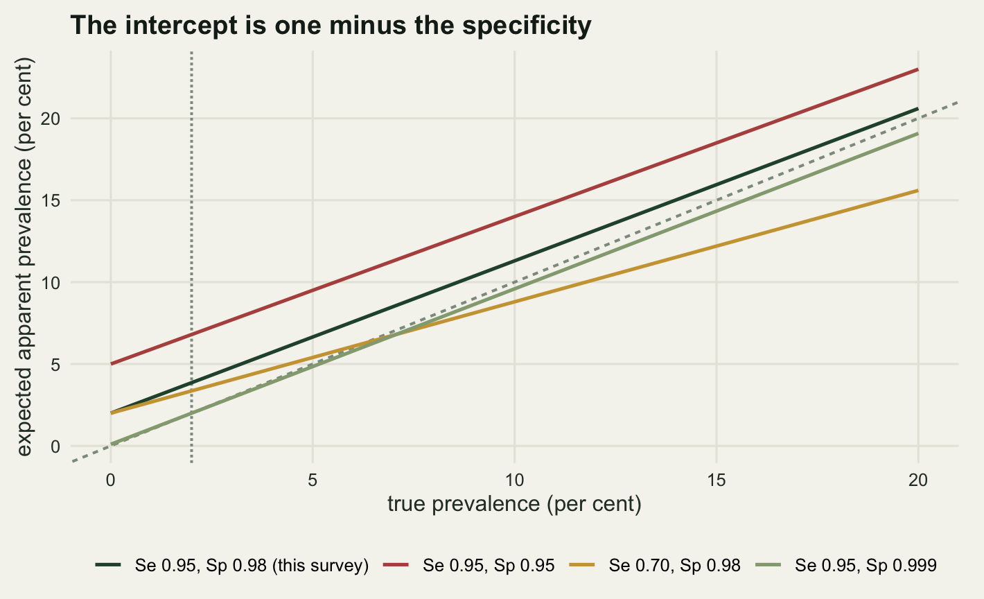
Every curve hits the vertical axis at \(1 - Sp\), because a population with no infection still produces false positives at that rate, and sensitivity only controls the slope. At the left-hand end of the panel, where wildlife disease surveys live, the curves separate by intercept, not slope.
The Rogan-Gladen correction
Inverting the mixture is one line. Rogan and Gladen (1978) set the observed apparent prevalence equal to its expectation and solved for \(p\):
\[\hat{p} = \frac{AP + Sp - 1}{Se + Sp - 1}\]
The denominator is the Youden index, 0.93 here, measuring how much of a change in true prevalence survives into the apparent prevalence; the numerator subtracts the false-positive floor. Both operations are linear, which makes the estimator easy and makes it behave badly at the boundary later on.
set.seed(20260804)
x_pos <- rbinom(1, n_survey, ap_exp)
ap_hat <- x_pos / n_survey
p_hat_one <- rg_of(ap_hat, se_true, sp_true)

print(c(positive_strips = x_pos, animals = n_survey))
positive_strips animals
23 480 print(round(c(apparent_prevalence = ap_hat,
corrected_prevalence = p_hat_one,
true_prevalence = p_true), 5)) apparent_prevalence corrected_prevalence true_prevalence
0.04792 0.03002 0.02000 One survey of 480 boar returns 23 positive strips, an apparent prevalence of 4.792 per cent, which the correction pulls back to 3.002 per cent against a truth of 2 per cent. Missing high on one draw is luck; landing on the truth on average is a property, and it takes a few thousand surveys to see.
n_rep <- 4000
set.seed(3311)
sv_known <- rbinom(n_rep, n_survey, ap_exp)
ap_known <- sv_known / n_survey
p_known <- rg_of(ap_known, se_true, sp_true)

print(round(c(mean_apparent = mean(ap_known), expected_apparent = ap_exp,
              mean_corrected = mean(p_known), true_prevalence = p_true,
              bias_of_apparent = mean(ap_known) - p_true,
              bias_of_corrected = mean(p_known) - p_true), 6))
mean_apparent expected_apparent mean_corrected true_prevalence
0.038639 0.038600 0.020042 0.020000
bias_of_apparent bias_of_corrected
0.018639 0.000042 print(round(c(mc_se_corrected = sd(p_known) / sqrt(n_rep), sd_corrected = sd(p_known),
sd_apparent = sd(ap_known), sd_ratio = sd(p_known) / sd(ap_known)), 6))mc_se_corrected sd_corrected sd_apparent sd_ratio
0.000148 0.009377 0.008721 1.075269 Over 4000 simulated surveys with the sensitivity and specificity known exactly, the apparent prevalence averages 3.8639 per cent and the corrected estimate averages 2.0042 per cent against a truth of 2, with a Monte Carlo standard error of 0.0148 percentage points. The correction is unbiased to the accuracy this can measure, and it divides the spread by the Youden index, so the standard deviation of the corrected estimate is 1.0753 times that of the apparent prevalence. That is the whole of the good news, and if the two test characteristics really were known constants the post could stop here.
The validation study is data too
They are not constants. Each came from one hundred animals and is a binomial proportion with its own sampling variation. One hundred negatives at a true specificity of 0.98 gives an expected two false positives in the panel, and the distribution of that count is not concentrated.
n_val_rep <- 20000
set.seed(6142)
sp_draws <- rbinom(n_val_rep, n_val_neg, sp_true) / n_val_neg
se_draws <- rbinom(n_val_rep, n_val_pos, se_true) / n_val_pos

print(round(c(mean_sp_hat = mean(sp_draws), sd_sp_hat = sd(sp_draws),
              mean_se_hat = mean(se_draws), sd_se_hat = sd(se_draws)), 5))
mean_sp_hat sd_sp_hat mean_se_hat sd_se_hat
0.98008 0.01392 0.94983 0.02181 print(round(c(sp_hat_equals_one = mean(sp_draws == 1),
sp_hat_at_or_below_0.96 = mean(sp_draws <= 0.96),
se_hat_equals_one = mean(se_draws == 1),
sp_hat_quantiles = quantile(sp_draws, c(0.025, 0.5, 0.975))), 4)) sp_hat_equals_one sp_hat_at_or_below_0.96 se_hat_equals_one
0.1335 0.1379 0.0060
sp_hat_quantiles.2.5% sp_hat_quantiles.50% sp_hat_quantiles.97.5%
0.9500 0.9800 1.0000 The estimated specificity has a standard deviation of 0.01392, and in 13.35 per cent of validation studies of this size the panel of one hundred negatives produces no false positives at all, so the reported specificity is exactly 1.00. That number comes back repeatedly below: a validation study reporting a perfect specificity has not demonstrated one, it has run out of resolution.
Propagating that into the corrected estimate needs the derivatives of the correction. Writing \(D = Se + Sp - 1\),
\[\frac{\partial \hat{p}}{\partial AP} = \frac{1}{D}, \qquad \frac{\partial \hat{p}}{\partial Se} = \frac{-\hat{p}}{D}, \qquad \frac{\partial \hat{p}}{\partial Sp} = \frac{1 - \hat{p}}{D}\]
so with the survey and the two validation arms independent, the delta-method variance is
\[\widehat{\operatorname{Var}}(\hat{p}) = \frac{1}{D^2}\left[ \frac{AP(1-AP)}{n} + \hat{p}^2\frac{Se(1-Se)}{n_{+}} + (1-\hat{p})^2\frac{Sp(1-Sp)}{n_{-}} \right]\]
The third term is the one that does the damage, because it carries the factor \((1-\hat{p})^2\), which at a prevalence of two per cent is essentially one.
delta_sd <- function(ap, se, sp, n, npos, nneg) {
  dd <- se + sp - 1
  ph <- (ap + sp - 1) / dd
  sqrt((ap * (1 - ap) / n + ph^2 * se * (1 - se) / npos +
          (1 - ph)^2 * sp * (1 - sp) / nneg) / dd^2)
}

v_survey <- ap_exp * (1 - ap_exp) / n_survey
v_sens <- p_true^2 * se_true * (1 - se_true) / n_val_pos
v_spec <- (1 - p_true)^2 * sp_true * (1 - sp_true) / n_val_neg
v_all <- v_survey + v_sens + v_spec
sd_fixed <- sqrt(v_survey) / youden
sd_full <- delta_sd(ap_exp, se_true, sp_true, n_survey, n_val_pos, n_val_neg)

print(round(100 * c(survey_share = v_survey, sensitivity_share = v_sens,
                    specificity_share = v_spec) / v_all, 4))
survey_share sensitivity_share specificity_share
29.0932 0.0715 70.8353 print(round(c(sd_treating_test_as_fixed = sd_fixed,
sd_carrying_validation = sd_full,
width_multiplier = sd_full / sd_fixed), 5))sd_treating_test_as_fixed sd_carrying_validation width_multiplier
0.00945 0.01753 1.85398 Split the variance three ways and the survey of 480 boar contributes 29.09 per cent of it, the sensitivity panel 0.071 per cent, and the specificity panel 70.84 per cent. The hundred known negatives are more than twice the source of uncertainty that the four hundred and eighty boar are. Standard errors follow: 0.00945 if the test characteristics are treated as fixed against 0.01753 if they are not, a multiplier of 1.854 on the width of every interval.
Coverage, measured
Three intervals go into the comparison, plus a reference case that could not be built in the field. The reference builds a Wilson (1927) interval for the apparent prevalence and pushes both endpoints through the correction using the true sensitivity and specificity, which separates the cost of the interval method from the cost of the validation study. The naive interval does the same with the estimated sensitivity and specificity substituted in and treated as constants, which is what gets published. The delta interval is the corrected estimate plus and minus 1.96 of the standard error above. The bootstrap resamples the survey and both validation arms from their fitted binomials. The Wilson form is used rather than Clopper and Pearson (1934) because the exact interval is conservative at these sample sizes and would flatter the naive method; nothing below turns on the choice.
zc <- qnorm(0.975)

wilson_ci <- function(x, n) {
  ph <- x / n
  cc <- (ph + zc^2 / (2 * n)) / (1 + zc^2 / n)
  hw <- zc * sqrt(ph * (1 - ph) / n + zc^2 / (4 * n^2)) / (1 + zc^2 / n)
  cbind(cc - hw, cc + hw)
}

boot_ci <- function(ap, se, sp, n, npos, nneg, n_boot) {
  aps <- rbinom(n_boot, n, ap) / n
  ses <- rbinom(n_boot, npos, se) / npos
  sps <- rbinom(n_boot, nneg, sp) / nneg
  ok <- ses + sps - 1 > 0
  qq <- quantile(rg_of(aps[ok], ses[ok], sps[ok]),
                 c(0.025, 0.975), names = FALSE)
  ph <- rg_of(ap, se, sp)
  c(percentile_lo = qq[1], percentile_hi = qq[2],
    basic_lo = 2 * ph - qq[2], basic_hi = 2 * ph - qq[1])
}
The sweep runs six true prevalences, two thousand surveys at each, each survey paired with its own fresh validation study of one hundred positives and one hundred negatives. Six hundred bootstrap resamples per survey is coarse for a tail quantile and it is enough for a coverage comparison at this resolution.
p_sweep <- c(0.005, 0.01, 0.02, 0.04, 0.08, 0.15)
n_cov <- 2000
n_boot <- 599
cov_tab <- data.frame(p = p_sweep)
head_line <- NULL

set.seed(7311)
for (k in seq_along(p_sweep)) {
  ap_k <- ap_of(p_sweep[k], se_true, sp_true)
  sv <- rbinom(n_cov, n_survey, ap_k)
  se_h <- rbinom(n_cov, n_val_pos, se_true) / n_val_pos
  sp_h <- rbinom(n_cov, n_val_neg, sp_true) / n_val_neg
  ap_h <- sv / n_survey
  wi <- wilson_ci(sv, n_survey)
  ph <- rg_of(ap_h, se_h, sp_h)
  sdv <- delta_sd(ap_h, se_h, sp_h, n_survey, n_val_pos, n_val_neg)

  lo_ref <- rg_of(wi[, 1], se_true, sp_true)
  hi_ref <- rg_of(wi[, 2], se_true, sp_true)
  lo_nai <- rg_of(wi[, 1], se_h, sp_h)
  hi_nai <- rg_of(wi[, 2], se_h, sp_h)
  lo_del <- ph - zc * sdv
  hi_del <- ph + zc * sdv
  bt <- matrix(NA_real_, n_cov, 4)
  for (i in seq_len(n_cov)) {
    bt[i, ] <- boot_ci(ap_h[i], se_h[i], sp_h[i],
                       n_survey, n_val_pos, n_val_neg, n_boot)
  }
  hit <- function(lo, hi) mean(lo <= p_sweep[k] & hi >= p_sweep[k])
  cov_tab$reference[k] <- hit(lo_ref, hi_ref)
  cov_tab$naive[k] <- hit(lo_nai, hi_nai)
  cov_tab$delta[k] <- hit(lo_del, hi_del)
  cov_tab$boot[k] <- hit(bt[, 3], bt[, 4])
  cov_tab$w_naive[k] <- mean(hi_nai - lo_nai)
  cov_tab$w_delta[k] <- mean(hi_del - lo_del)
  cov_tab$w_boot[k] <- mean(bt[, 4] - bt[, 3])
  if (p_sweep[k] == p_true) {
    head_line <- list(ph = ph, sdv = sdv, sp_h = sp_h, se_h = se_h,
                      lo_nai = lo_nai, hi_nai = hi_nai,
                      lo_del = lo_del, hi_del = hi_del, bt = bt)
  }
}
print(round(cov_tab, 4))
p reference naive delta boot w_naive w_delta w_boot
1 0.005 0.9470 0.6080 0.8750 0.8800 0.0304 0.0633 0.0631
2 0.010 0.9510 0.6215 0.8760 0.8765 0.0331 0.0652 0.0651
3 0.020 0.9385 0.7030 0.9085 0.9120 0.0376 0.0668 0.0668
4 0.040 0.9530 0.7710 0.9295 0.9335 0.0450 0.0713 0.0713
5 0.080 0.9455 0.8320 0.9395 0.9485 0.0562 0.0771 0.0772
6 0.150 0.9495 0.8765 0.9475 0.9535 0.0704 0.0876 0.0876hl <- head_line
in_ok <- function(lo, hi) lo <= p_true & hi >= p_true
row_at <- which(cov_tab$p == p_true)
cov_ref <- cov_tab$reference[row_at]
cov_nai <- cov_tab$naive[row_at]
cov_del <- cov_tab$delta[row_at]
cov_boo <- cov_tab$boot[row_at]
cov_pct <- mean(in_ok(hl$bt[, 1], hl$bt[, 2]))
print(round(c(reference_known_test = cov_ref, naive_fixed = cov_nai,
delta_propagated = cov_del, bootstrap_basic = cov_boo,
bootstrap_percentile = cov_pct), 4))reference_known_test naive_fixed delta_propagated
0.9385 0.7030 0.9085
bootstrap_basic bootstrap_percentile
0.9120 0.8925 print(round(c(naive_miss_low = mean(hl$lo_nai > p_true),
naive_miss_high = mean(hl$hi_nai < p_true),
delta_miss_low = mean(hl$lo_del > p_true),
delta_miss_high = mean(hl$hi_del < p_true),
lower_limit_below_zero = mean(hl$lo_del < 0)), 4)) naive_miss_low naive_miss_high delta_miss_low
0.1895 0.1075 0.0880
delta_miss_high lower_limit_below_zero
0.0035 0.6685 print(round(c(width_naive = cov_tab$w_naive[row_at], width_delta = cov_tab$w_delta[row_at],
width_ratio = cov_tab$w_delta[row_at] / cov_tab$w_naive[row_at]), 4))width_naive width_delta width_ratio
0.0376 0.0668 1.7778 At the design prevalence of 2 per cent the reference interval covers the truth 93.85 per cent of the time, close enough to the nominal rate to confirm the machinery. Substituting the estimated sensitivity and specificity and carrying on as though they were exact takes coverage to 70.3 per cent: a nominal ninety-five per cent interval that misses one time in three, with 18.95 per cent of surveys returning an interval entirely above the truth and 10.75 per cent entirely below.
Propagating the validation study restores most of it. The delta interval covers 90.85 per cent and the bootstrap 91.2 per cent, and the price is width: 0.0668 against 0.0376, a factor of 1.778. The honest interval on a two per cent prevalence is about 6.68 percentage points wide, and its lower limit is below zero in 66.85 per cent of surveys.
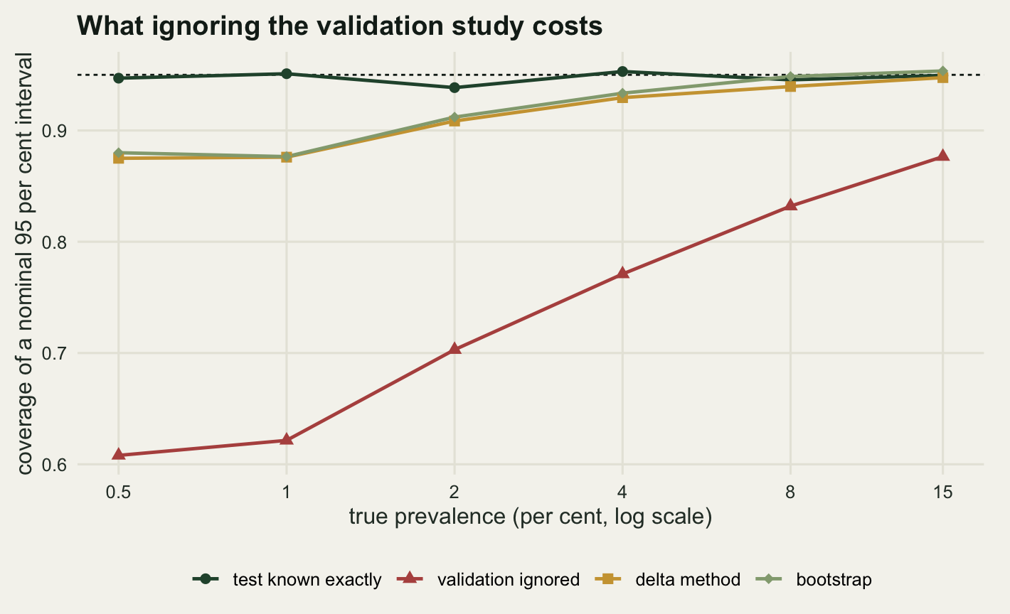
Coverage of the naive interval is worst where the survey is most likely to be run: at a true prevalence of 0.5 per cent it covers 60.8 per cent of the time, climbing only to 87.65 per cent at 15 per cent, where the survey uncertainty has grown large enough to hide the validation uncertainty inside it.
Where the delta method and the bootstrap part company
On the summary above the two propagated intervals are interchangeable. Their coverages differ by less than a percentage point at every prevalence in the sweep and their mean widths agree to three decimal places. They differ in two places that the summary hides.
sp_one <- hl$sp_h == 1
skew_ph <- mean((hl$ph - mean(hl$ph))^3) / sd(hl$ph)^3
shift_lo <- mean(hl$bt[, 3] - hl$bt[, 1])

print(round(c(skewness_of_corrected = skew_ph, percentile_coverage = cov_pct,
              basic_coverage = cov_boo, lower_limit_shift = shift_lo,
              mean_abs_endpoint_gap = mean(abs(hl$lo_del - hl$bt[, 3]))), 5))
skewness_of_corrected percentile_coverage basic_coverage
-0.40894 0.89250 0.91200
lower_limit_shift mean_abs_endpoint_gap
0.00669 0.00366 by_panel <- function(sel) c(
share = mean(sel),
delta_cover = mean(in_ok(hl$lo_del, hl$hi_del)[sel]),
boot_cover = mean(in_ok(hl$bt[, 3], hl$bt[, 4])[sel]),
delta_width = mean((hl$hi_del - hl$lo_del)[sel]))
print(round(rbind(sp_hat_one = by_panel(sp_one),
sp_hat_below_one = by_panel(!sp_one)), 4)) share delta_cover boot_cover delta_width
sp_hat_one 0.1295 0.3822 0.4247 0.0364
sp_hat_below_one 0.8705 0.9868 0.9845 0.0713The first disagreement is about which end of the bootstrap distribution to use. The sampling distribution of the corrected estimate is left skewed, with a skewness of -0.409, inherited from the estimated specificity: \(\hat{Sp}\) is bounded above by one, piles up near the boundary and tails away downwards, and \(\hat{p}\) increases in \(\hat{Sp}\). The percentile interval, which reports the quantiles of the bootstrap distribution directly, therefore sits low, its lower limit 0.00669 below the basic interval’s on average. That shift is worth 91.2 per cent coverage for the basic form against 89.25 per cent for the percentile form, which is the one people reach for first.
The second disagreement is not between the two methods but between both of them and the world. Split the two thousand surveys by whether the validation panel produced a specificity of exactly 1.00. Where it did not, in 87.05 per cent of surveys, the delta interval covers 98.68 per cent of the time and the bootstrap 98.45 per cent, both well above nominal. Where it did, in 12.95 per cent of surveys, coverage falls to 38.22 per cent and 42.47 per cent respectively.
Both methods fail in the same place for the same reason. A validation panel with no false positives gives \(\hat{Sp}(1-\hat{Sp})/n_{-} = 0\), so the delta method assigns the specificity no uncertainty at all and the interval narrows to 0.0364 from 0.0713; the parametric bootstrap resamples from \(\hat{Sp} = 1\) and every resample also has a perfect specificity, so it inherits the same blind spot. The overall 90.85 per cent is therefore not a well-behaved interval but a mixture of one that over-covers badly and one that covers less than half the time, and which a given survey gets is decided by a Binomial draw in a validation study that may have happened years earlier.
Negative prevalence
The correction is a linear inversion and nothing in it is bounded. The numerator \(AP + Sp - 1\) goes negative whenever the observed apparent prevalence falls below the false-positive rate of the test, and there is no reason it should not: if the pathogen is rare enough, a survey can easily produce fewer positive strips than the test would have produced from an uninfected population.
p_grid <- c(0, 0.005, 0.01, 0.02, 0.03, 0.05)
n_grid <- c(120, 240, 480, 960, 1920)
n_neg_rep <- 4000
neg_tab <- expand.grid(p = p_grid, n = n_grid)
neg_tab$known <- NA_real_
neg_tab$estimated <- NA_real_

set.seed(5510)
for (k in seq_len(nrow(neg_tab))) {
  ap_k <- ap_of(neg_tab$p[k], se_true, sp_true)
  ap_d <- rbinom(n_neg_rep, neg_tab$n[k], ap_k) / neg_tab$n[k]
  se_d <- rbinom(n_neg_rep, n_val_pos, se_true) / n_val_pos
  sp_d <- rbinom(n_neg_rep, n_val_neg, sp_true) / n_val_neg
  neg_tab$known[k] <- mean(rg_of(ap_d, se_true, sp_true) < 0)
  neg_tab$estimated[k] <- mean(rg_of(ap_d, se_d, sp_d) < 0)
}
print(round(neg_tab[neg_tab$n %in% c(120, 480, 1920), ], 4))
p n known estimated
1 0.000 120 0.5800 0.5155
2 0.005 120 0.4345 0.4052
3 0.010 120 0.3005 0.3220
4 0.020 120 0.1550 0.2040
5 0.030 120 0.0665 0.1128
6 0.050 120 0.0110 0.0312
13 0.000 480 0.5075 0.4550
14 0.005 480 0.2560 0.3470
15 0.010 480 0.1020 0.2545
16 0.020 480 0.0090 0.1355
17 0.030 480 0.0005 0.0605
18 0.050 480 0.0000 0.0082
25 0.000 1920 0.5038 0.4582
26 0.005 1920 0.0968 0.3302
27 0.010 1920 0.0063 0.2422
28 0.020 1920 0.0000 0.1098
29 0.030 1920 0.0000 0.0428
30 0.050 1920 0.0000 0.0050pick <- function(pp, nn, col) neg_tab[[col]][neg_tab$p == pp & neg_tab$n == nn]
print(round(c(at_zero_n120 = pick(0, 120, "known"), at_zero_n1920 = pick(0, 1920, "known"),
at_two_pct_n120_known = pick(0.02, 120, "known"),
at_two_pct_n1920_known = pick(0.02, 1920, "known"),
at_two_pct_n120_est = pick(0.02, 120, "estimated"),
at_two_pct_n1920_est = pick(0.02, 1920, "estimated"),
at_one_pct_n1920_est = pick(0.01, 1920, "estimated")), 4)) at_zero_n120 at_zero_n1920 at_two_pct_n120_known
0.5800 0.5038 0.1550
at_two_pct_n1920_known at_two_pct_n120_est at_two_pct_n1920_est
0.0000 0.2040 0.1098
at_one_pct_n1920_est
0.2422 With the specificity known exactly the frequency of a negative estimate behaves the way intuition says it should, for every prevalence except one. At a true prevalence of 2 per cent it falls from 15.5 per cent of surveys at 120 animals to 0 per cent at 1920. The exception is a genuinely uninfected population, where the expected apparent prevalence is exactly \(1 - Sp\) and the observed one falls below it about half the time whatever the sample size: 58 per cent at 120 animals and 50.38 per cent at 1920. No survey effort will move that, because the estimator stays centred on zero however many animals are sampled. The positive count is discrete and right skewed, most strongly in the smallest surveys, so the frequency wobbles around a half rather than sitting on it. With the specificity estimated, sample size stops helping much earlier.
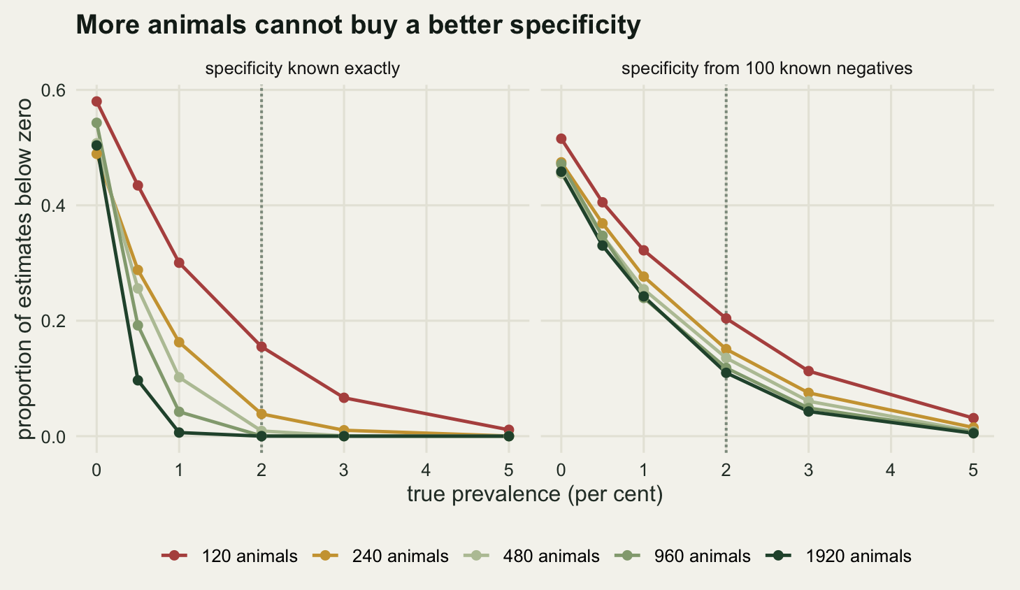
The right-hand panel is the finding. At a true prevalence of 2 per cent, which is exactly \(1 - Sp\) for this test, the frequency of a negative estimate goes from 20.4 per cent at 120 animals to 10.97 per cent at 1920. Sixteen times the fieldwork buys a reduction of 9.42 percentage points, and that is as low as it goes. A larger survey pushes the frequency back up towards 13.79 per cent, the share of validation panels reporting a specificity of 0.96 or below, whose own false-positive rate already exceeds the expected apparent prevalence of 3.86 per cent. The limit belongs to the hundred known negatives, not to the survey. At half that prevalence the picture is worse: one survey in four returns a negative estimate at 1920 animals, against 0.62 per cent when the specificity is known.
A negative estimate is not a mistake. It says the survey saw fewer positives than an uninfected population of that size would be expected to produce, which is an ordinary thing for data to say when the pathogen is rare or absent. The estimator returns a number outside the parameter space because it is a linear inversion and nothing in the arithmetic knows that prevalence lives in \([0, 1]\).
The cost of truncating at zero
The usual response is to report zero. That is defensible as a statement about the parameter and it changes the estimator, so the change should be measured rather than assumed harmless.
p_low <- c(0, 0.0025, 0.005, 0.01, 0.02)
n_tr_rep <- 4000
tr_tab <- data.frame(p = p_low)
tr_draws <- NULL

set.seed(8810)
for (k in seq_along(p_low)) {
  ap_k <- ap_of(p_low[k], se_true, sp_true)
  ap_d <- rbinom(n_tr_rep, n_survey, ap_k) / n_survey
  se_d <- rbinom(n_tr_rep, n_val_pos, se_true) / n_val_pos
  sp_d <- rbinom(n_tr_rep, n_val_neg, sp_true) / n_val_neg
  ph <- rg_of(ap_d, se_d, sp_d)
  sdv <- delta_sd(ap_d, se_d, sp_d, n_survey, n_val_pos, n_val_neg)
  pt <- pmax(ph, 0)
  lo <- ph - zc * sdv
  hi <- ph + zc * sdv
  tr_tab$raw_mean[k] <- mean(ph); tr_tab$trunc_mean[k] <- mean(pt)
  tr_tab$rmse_raw[k] <- sqrt(mean((ph - p_low[k])^2))
  tr_tab$rmse_trunc[k] <- sqrt(mean((pt - p_low[k])^2))
  tr_tab$cover_raw[k] <- mean(lo <= p_low[k] & hi >= p_low[k])
  tr_tab$cover_clip[k] <- mean(pmax(lo, 0) <= p_low[k] & pmax(hi, 0) >= p_low[k])
  tr_tab$width_raw[k] <- mean(hi - lo)
  tr_tab$width_clip[k] <- mean(pmax(hi, 0) - pmax(lo, 0))
  tr_tab$q90_trunc[k] <- unname(quantile(pt, 0.9))
  tr_tab$mc_se[k] <- sd(ph) / sqrt(n_tr_rep)
  tr_tab$at_design[k] <- mean(pt >= p_true)
  if (p_low[k] == 0) tr_draws <- ph
}
print(round(tr_tab[, 1:6], 5))
p raw_mean trunc_mean rmse_raw rmse_trunc cover_raw
1 0.0000 -0.00032 0.00635 0.01640 0.01054 0.87275
2 0.0025 0.00288 0.00825 0.01668 0.01123 0.85675
3 0.0050 0.00491 0.00963 0.01681 0.01145 0.87425
4 0.0100 0.00960 0.01292 0.01717 0.01238 0.89650
5 0.0200 0.01974 0.02106 0.01721 0.01472 0.90925print(round(tr_tab[, c(1, 7:12)], 5)) p cover_clip width_raw width_clip q90_trunc mc_se at_design
1 0.0000 0.87450 0.06269 0.03002 0.01958 0.00026 0.09000
2 0.0025 0.85675 0.06221 0.03259 0.02264 0.00026 0.14700
3 0.0050 0.87425 0.06347 0.03507 0.02551 0.00027 0.19600
4 0.0100 0.89650 0.06517 0.04007 0.02990 0.00027 0.29025
5 0.0200 0.90925 0.06687 0.04895 0.04123 0.00027 0.51975Start with the point estimate in a population that genuinely has none of the virus. The untruncated estimator averages -0.0316 per cent, against a Monte Carlo standard error of 0.0259 percentage points, so it is sitting on zero. Truncating at zero takes the average of what gets reported to 0.6348 per cent. The ninetieth percentile of what it reports is 1.958 per cent, and in 9 per cent of these surveys the reported prevalence is at or above the 2 per cent the survey was designed to detect, in a population where the pathogen is absent.
The bias decays as the pathogen becomes commoner but not quickly. At a true prevalence of 0.5 per cent the truncated estimator averages 0.963 per cent, and at 2 per cent it averages 2.106 per cent, still 0.106 percentage points high.
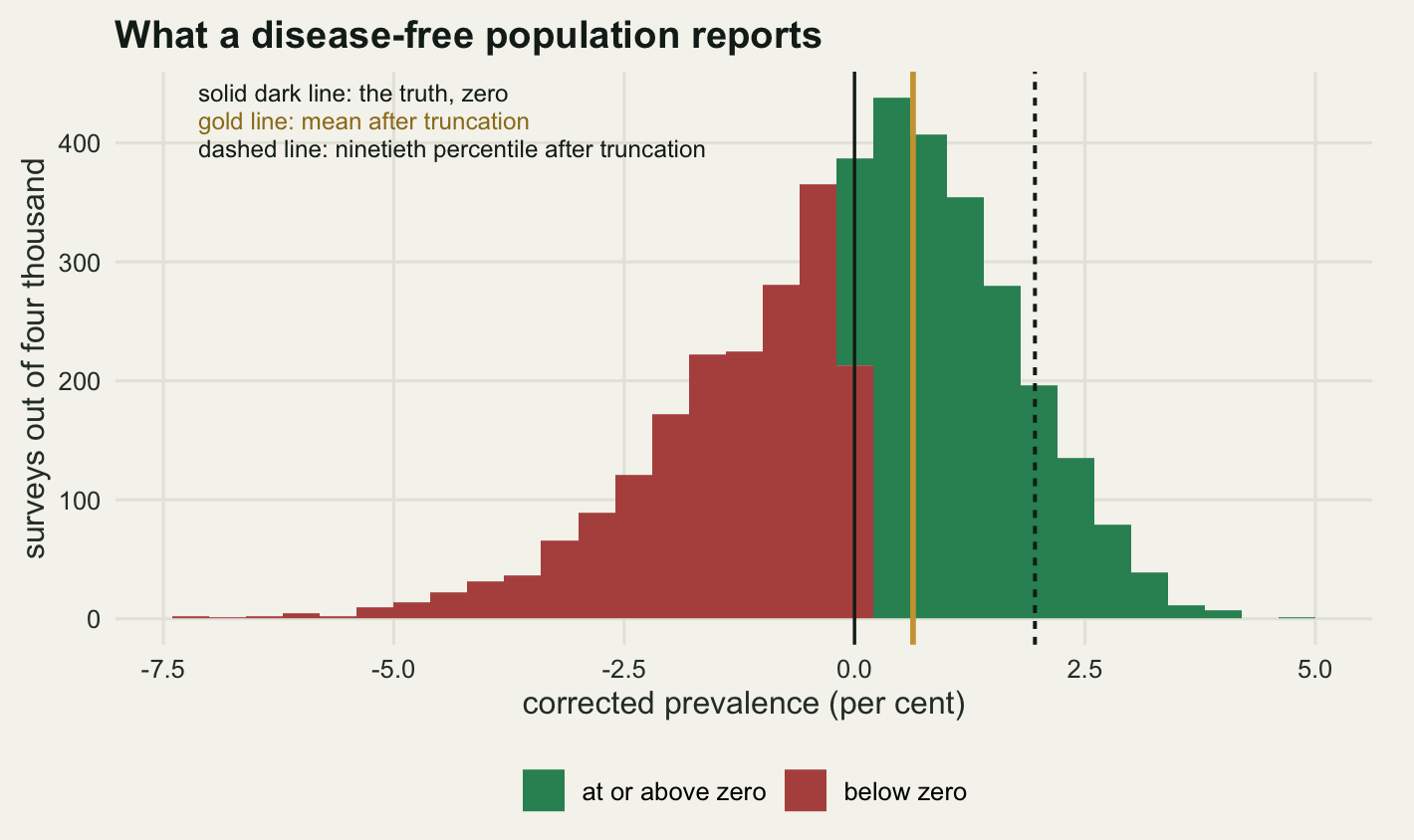
Two things about truncation came out differently from what I expected before running it.
It improves mean squared error, and by a wide margin. At a true prevalence of zero the root mean squared error falls from 1.64 percentage points to 1.054, and it is lower at every prevalence in the table. That is not a surprise once stated: pushing an estimate towards a boundary the parameter cannot cross is shrinkage, and shrinkage buys variance at the cost of bias. Anyone choosing between the two estimators on squared error alone should truncate.
It does not damage interval coverage either, and cannot. Clipping the interval to \([\max(lo, 0), \max(hi, 0)]\) leaves coverage at 87.45 per cent against 87.28 per cent unclipped at zero prevalence, and identical to four decimal places at every positive prevalence tested. The reason is arithmetic rather than luck: if the true value is non-negative and the original interval covered it, no part of the interval below zero was doing any work.
What truncation is not free in is width. The clipped interval at zero prevalence averages 3.002 percentage points against 6.269 unclipped, so a reader sees an interval 52.1 per cent narrower with no gain in information. Put the two together and the truncated report is a point estimate biased upwards by 0.635 percentage points attached to an interval that looks twice as precise as the honest one. That combination is worse than either part, and it is the standard output.
Specificity sets the floor, not sample size
The design question a survey like this exists to answer is usually not “what is the prevalence” but “is the pathogen here at all”, a test of \(p = 0\). Cameron and Baldock (1998) built the standard freedom-from-disease sample size calculation for exactly this question. The version below asks something more demanding: how many animals are needed for the 95 per cent interval on the corrected prevalence to exclude zero, with probability 0.8, when the truth is 2 per cent. Under \(p = 0\) the expected apparent prevalence is \(1 - Sp\), and under the alternative it is \(Se \cdot p + (1 - Sp)(1 - p)\); the gap between them is \(p \cdot D\), the true prevalence shrunk by the Youden index. The variance that gap has to beat has two parts, one that shrinks with the survey and one that does not.
req_n <- function(p, se, sp, nneg, pow = 0.8) {
  ap1 <- ap_of(p, se, sp)
  sig_target <- p * (se + sp - 1) / (zc + qnorm(pow))
  budget <- sig_target^2 - sp * (1 - sp) / nneg
  ifelse(budget <= 0, NA_real_, ap1 * (1 - ap1) / budget)
}

min_neg <- function(p, se, sp, pow = 0.8) {
  sp * (1 - sp) / (p * (se + sp - 1) / (zc + qnorm(pow)))^2
}
pow_ceiling <- function(p, se, sp, nneg) {
  pnorm(p * (se + sp - 1) / sqrt(sp * (1 - sp) / nneg) - zc)
}

sp_show <- c(0.95, 0.96, 0.97, 0.98, 0.99, 0.995, 0.999)
des_tab <- data.frame(
  specificity = sp_show,
  n_if_known = req_n(p_true, se_true, sp_show, Inf),
  n_val_2000 = req_n(p_true, se_true, sp_show, 2000),
  n_val_500 = req_n(p_true, se_true, sp_show, 500),
  n_val_100 = req_n(p_true, se_true, sp_show, 100),
  min_negatives = min_neg(p_true, se_true, sp_show),
  ceiling_100 = pow_ceiling(p_true, se_true, sp_show, 100))
print(round(des_tab, 2))
specificity n_if_known n_val_2000 n_val_500 n_val_100 min_negatives
1 0.95 1535.28 3615.33 NA NA 1150.68
2 0.96 1298.81 2382.94 NA NA 909.91
3 0.97 1067.76 1611.26 NA NA 674.63
4 0.98 841.92 1082.63 7608.21 NA 444.67
5 0.99 621.15 697.86 1108.60 NA 219.85
6 1.00 512.60 542.23 656.02 NA 109.31
7 1.00 426.62 431.32 446.04 545.32 21.77
ceiling_100
1 0.13
2 0.15
3 0.19
4 0.26
5 0.47
6 0.76
7 1.00sp_break <- uniroot(function(s) min_neg(p_true, se_true, s) - n_val_neg,
c(0.98, 0.9999))$root
sp_for_480 <- uniroot(function(s) req_n(p_true, se_true, s, Inf) - n_survey,
c(0.98, 0.9999))$root
print(round(c(specificity_making_100_negatives_enough = sp_break,
specificity_making_480_animals_enough = sp_for_480,
min_negatives_at_design_spec = min_neg(p_true, se_true, sp_true),
power_ceiling_at_design_spec =
pow_ceiling(p_true, se_true, sp_true, n_val_neg)), 5))specificity_making_100_negatives_enough specificity_making_480_animals_enough
0.99542 0.99651
min_negatives_at_design_spec power_ceiling_at_design_spec
444.67003 0.26389 The first column is the classical answer: with the specificity known exactly, distinguishing a two per cent prevalence from zero needs 842 animals at a specificity of 0.98, 1535 at 0.95 and 427 at 0.999. Improving the test from 0.95 to 0.99 specificity does the work of 2.47 times the fieldwork. That alone is the design lesson people usually take away.
The rest of the table does not appear in a standard calculation. With the specificity estimated from a panel of 100 known negatives, the sample size at 0.98 specificity is not large. It does not exist. The validation variance does not shrink when animals are added, so once it alone exceeds what the design can tolerate, no survey size will do. The ceiling on power at 0.98 specificity with 100 validation negatives is 26.39 per cent, reached in the limit of infinitely many animals.
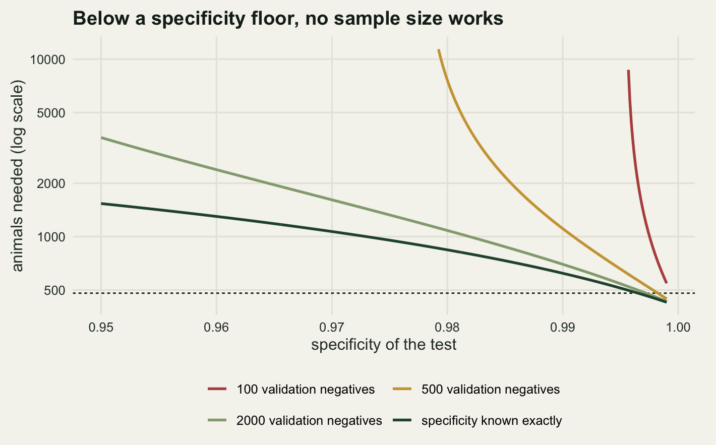
Read the figure as a set of walls. With 100 known negatives in the validation panel the design is impossible until the specificity passes 0.9954; with five hundred the wall moves left; with the specificity known exactly there is no wall at all and the curve is a smooth trade against sample size. Turning that round gives the number a survey planner needs: at the design specificity of 0.98, the validation panel needs at least 445 known negatives before any survey size can distinguish a two per cent prevalence from zero. The panel of 100 was short by a factor of about 4.4.
The closed form uses the variance under the alternative for both hypotheses, which makes it conservative, and the plug-in test is not correctly sized when the validation panel is small. Both are worth measuring rather than asserting.
sim_reject <- function(nn, nneg, p_at, reps = 40000, seed = 4400) {
  set.seed(seed)
  ap_d <- rbinom(reps, nn, ap_of(p_at, se_true, sp_true)) / nn
  se_d <- rbinom(reps, n_val_pos, se_true) / n_val_pos
  sp_d <- if (is.finite(nneg)) rbinom(reps, nneg, sp_true) / nneg else
    rep(sp_true, reps)
  nv <- if (is.finite(nneg)) nneg else 1e12
  ph <- rg_of(ap_d, se_d, sp_d)
  mean(ph - zc * delta_sd(ap_d, se_d, sp_d, nn, n_val_pos, nv) > 0)
}

n_formula <- ceiling(req_n(p_true, se_true, sp_true, Inf))
pow_grid <- c(650, 700, 750, 800, n_formula)
print(rbind(animals = pow_grid,
            power = round(vapply(pow_grid,
                                 function(nn) sim_reject(nn, Inf, p_true),
                                 numeric(1)), 4)))
[,1] [,2] [,3] [,4] [,5]
animals 650.0000 700.0000 750.0000 800.0000 842.0000
power 0.6952 0.7528 0.8022 0.8384 0.8582size_grid <- c(100, 250, 500, 1000, 2000)
print(rbind(validation_negatives = size_grid,
size_at_p_zero = round(vapply(size_grid,
function(nv) sim_reject(n_survey, nv, 0),
numeric(1)), 4))) [,1] [,2] [,3] [,4] [,5]
validation_negatives 100.0000 250.000 500.0000 1.00e+03 2.00e+03
size_at_p_zero 0.1334 0.047 0.0251 1.55e-02 1.07e-02print(round(c(size_with_known_specificity = sim_reject(n_survey, Inf, 0)), 4))size_with_known_specificity
0.0091 The formula asks for 842 animals and simulation puts the true requirement near 750, where power is 0.8022, so the closed form is conservative by roughly 12 per cent. Use it as a design number and expect to be slightly over-resourced, which is the right direction to be wrong in.
The size of the test is the more serious problem. At 480 animals and a validation panel of 100 negatives, the delta-method interval excludes zero in a genuinely uninfected population 13.33 per cent of the time against a nominal 2.5. The cause is the one already identified: when the validation panel records no false positives, the specificity term in the variance vanishes, the interval collapses, and its lower limit sits above zero. That failure rate is essentially the 13.35 per cent chance of a clean validation panel. With five hundred validation negatives the size falls to 2.51 per cent and with the specificity known to 0.9 per cent. A small validation study does not merely widen the answer; it manufactures detections of a pathogen that is not there.
The honest limit
Everything above treats the sensitivity and the specificity as fixed properties of the test, uncertain only through the size of the validation panel. That is the assumption the whole correction rests on and it is the weakest thing here.
Validation panels are assembled from animals whose status is known, which usually means clinically affected animals with high antibody titres on the positive side and animals from a region with no history of the pathogen on the negative side. The sensitivity measured that way is the sensitivity against strong positives, and the survey will contain early infections and recovering animals that the strip finds less often. Greiner and Gardner (2000) set out this spectrum problem and the validation design literature that goes with it. If field sensitivity is lower than the panel’s, the correction under-corrects; if field specificity is lower, every number in this post is optimistic. Neither direction can be checked from the survey data, because the survey has no gold standard in it. That is what makes it a survey.
Three further assumptions are load-bearing. Test errors are treated as independent between animals, so a bad reagent lot or one operator with a systematic reading habit would make false positives cluster and the effective validation panel smaller than one hundred, which makes every interval above too narrow rather than too wide. The reference assay is treated as a true gold standard; when it is not, the two numbers are relative sensitivity and relative specificity, and a latent class model with two imperfect tests is the honest formulation. And the survey is treated as a simple random sample, which hunter-submitted samples are not: Nusser, Clark, Otis and Huang (2008) show what convenience sampling does to a wildlife disease prevalence estimate, and that bias sits on top of everything measured here.
The delta method and the parametric bootstrap were used because they are what an ecologist would build from base R in an afternoon, and they share a boundary failure that neither can see. Reiczigel, Foldi and Ozsvari (2010) and Lang and Reiczigel (2014) give intervals for true prevalence that behave properly there, the second of them specifically for estimated sensitivity and specificity, and either is a better production choice than the code above.
Where to go next
The clean fix for the boundary is not truncation but a model that never leaves the parameter space. A prior on \(p\) supported on \([0, 1]\), with priors on \(Se\) and \(Sp\) carrying the validation counts, gives a posterior that is bounded by construction, propagates the validation uncertainty without a delta approximation, and degrades gracefully when the panel reports a perfect specificity, because a Beta posterior from 100 negatives and zero false positives still has a tail. The cost is that the answer near zero prevalence is then partly a statement about the prior, which is exactly the information the data did not have.
The other direction is dropping the gold standard. Two imperfect tests applied to the same animals across two populations with different prevalences identify all the parameters without any validation panel, which turns the problem from correction into estimation and removes the transfer assumption this post could not check.
References
Rogan WJ, Gladen B 1978 American Journal of Epidemiology 107(1):71-76 (10.1093/oxfordjournals.aje.a112510)
Wilson EB 1927 Journal of the American Statistical Association 22(158):209-212 (10.1080/01621459.1927.10502953)
Clopper CJ, Pearson ES 1934 Biometrika 26(4):404-413 (10.1093/biomet/26.4.404)
Cameron AR, Baldock FC 1998 Preventive Veterinary Medicine 34(1):1-17 (10.1016/S0167-5877(97)00081-0)
Greiner M, Gardner IA 2000 Preventive Veterinary Medicine 45(1-2):3-22 (10.1016/S0167-5877(00)00114-8)
Nusser SM, Clark WR, Otis DL, Huang L 2008 The Journal of Wildlife Management 72(1):52-60 (10.2193/2007-317)
Reiczigel J, Foldi J, Ozsvari L 2010 Epidemiology and Infection 138(11):1674-1678 (10.1017/S0950268810000385)
Lang Z, Reiczigel J 2014 Preventive Veterinary Medicine 113(1):13-22 (10.1016/j.prevetmed.2013.09.015)