library(ggplot2)
library(grid)

te_ink <- "#16241d"; te_forest <- "#275139"; te_gold <- "#c9b458"
te_rust <- "#b5534e"; te_sage <- "#93a87f"

theme_te <- function() {
  theme_minimal(base_size = 11) +
    theme(
          plot.background  = element_rect(fill = "#f5f4ee", colour = NA),
          panel.background = element_rect(fill = "#f5f4ee", colour = NA),
          panel.grid.minor = element_blank(),
          panel.grid.major = element_line(colour = "grey90", linewidth = 0.3),
          plot.title = element_text(colour = te_ink, face = "bold", size = 11),
          plot.subtitle = element_text(colour = "grey35", size = 9),
          axis.title = element_text(colour = te_ink, size = 9),
          axis.text = element_text(colour = "grey30", size = 8),
          legend.position = "bottom",
          legend.title = element_blank(),
          legend.text = element_text(size = 8))
}
two_panel <- function(p1, p2) {
  grid.newpage()
  pushViewport(viewport(layout = grid.layout(1, 2)))
  print(p1, vp = viewport(layout.pos.row = 1, layout.pos.col = 1))
  print(p2, vp = viewport(layout.pos.row = 1, layout.pos.col = 2))
}False positives in occupancy models
R
occupancy
imperfect detection
ecology tutorial
Why a five per cent misidentification rate inflates an occupancy estimate in R, and how the label swap leaves two answers that fit the detection data alike.
Corrected 1 October 2026: the post said BFGS walks the Royle-Nichols likelihood onto a boundary; in that post it is the standard occupancy likelihood that does so. It also gave the wrong condition for the constraint on the two detection rates to fail, and the sweep now fits the false-positive model from two starts with the labels set by that constraint.
Updated 25 September 2026: the comparison with the Royle-Nichols model now matches that post’s new section on calibration counts.
The standard occupancy model rests on an assumption so quiet that it is easy to miss: you can fail to see a species that is there, but you can never see a species that is not. Every correction the model applies runs in one direction. It assumes silence is evidence of nothing.
Break that assumption slightly, at a rate of one visit in twenty, and the model does not degrade gracefully. It reports occupancy several times the truth.
A rare species and a fallible observer
Two hundred and fifty sites, five visits, a species present at one site in ten. When it is there you record it on 35% of visits. When it is not there you record it anyway on 5% of visits, because a similar call carries across the valley, or a footprint is ambiguous, or the automated classifier has a bad day.
set.seed(4274)
R <- 250L; K <- 5L
psi_t <- 0.10; p11_t <- 0.35; p10_t <- 0.05
z <- rbinom(R, 1L, psi_t)
Y <- matrix(rbinom(R * K, 1L, ifelse(rep(z, K) == 1, p11_t, p10_t)), R, K)
d <- rowSums(Y)

occupied <- sum(z)
detected <- sum(d > 0)
false_sites <- sum(d > 0 & z == 0)
naive <- mean(d > 0)
The species truly occupies 22 of the 250 sites. It was recorded at least once at 73 sites, of which 55 hold no species at all. The naive estimate is 0.2920 against a truth of 0.10.
A careful analyst knows the naive estimate is biased and reaches for the correction.
ct <- list(maxit = 8000, reltol = 1e-12)
fit_nm <- function(nll, start, se = TRUE, ...) {
  o <- optim(start, nll, ..., method = "Nelder-Mead", control = ct)
  o <- optim(o$par, nll, ..., method = "Nelder-Mead", control = ct)
  s <- rep(NA_real_, length(o$par))
  if (se) {
    H <- optimHess(o$par, nll, ...)
    s <- tryCatch(sqrt(diag(solve(H))),
                  error = function(e) rep(NA_real_, length(o$par)))
  }
  list(par = o$par, se = s, nll = o$value,
       aic = 2 * o$value + 2 * length(o$par))
}
occ_nll <- function(par, d, K) {
  psi <- plogis(par[1]); p <- plogis(par[2])
  pd <- psi * dbinom(0:K, K, p) + c(1 - psi, rep(0, K))
  -sum(log(pmax(pd[d + 1], 1e-300)))
}
fp_nll <- function(par, d, K) {
  psi <- plogis(par[1]); p11 <- plogis(par[2]); p10 <- plogis(par[3])
  pd <- psi * dbinom(0:K, K, p11) + (1 - psi) * dbinom(0:K, K, p10)
  -sum(log(pmax(pd[d + 1], 1e-300)))
}
f_occ <- fit_nm(occ_nll, c(0, 0), d = d, K = K)
f_fp <- fit_nm(fp_nll, c(0, qlogis(0.4), qlogis(0.05)), d = d, K = K)

psi_occ <- plogis(f_occ$par[1])
ci_occ <- plogis(f_occ$par[1] + c(-1.96, 1.96) * f_occ$se[1])
psi_fp <- plogis(f_fp$par[1])
ci_fp <- plogis(f_fp$par[1] + c(-1.96, 1.96) * f_fp$se[1])
implied_missed <- R * psi_occ - detected
The standard occupancy model reports \(\hat\psi = 0.5752\), a 95% interval of [0.383, 0.747], against a truth of 0.10. It is not slightly wrong. It is wrong by a factor of 5.8.
The mechanism is worth stating plainly, because it is the opposite of what intuition suggests. The model sees 73 sites with detections and a fitted detection probability of only 0.132. Low detection means many occupied sites must have been missed entirely, so the model adds them: it infers roughly 71 occupied-but-never-detected sites, when the true number of such sites is 4. The correction for false negatives amplifies the false positives. A scatter of spurious single detections looks exactly like a real species that is hard to see, and the model responds by concluding the species is everywhere and shy.
Royle and Link (2006) add one parameter. Detection is a two-component mixture: occupied sites detect at \(p_{11}\), unoccupied sites detect at \(p_{10}\).
\[\Pr(d_i) = \psi \binom{K}{d_i} p_{11}^{d_i}(1-p_{11})^{K-d_i} + (1-\psi)\binom{K}{d_i} p_{10}^{d_i}(1-p_{10})^{K-d_i}\]
The standard model is the special case \(p_{10} = 0\). That is the entire difference.
p11_hat <- plogis(f_fp$par[2]); p10_hat <- plogis(f_fp$par[3])Fitted, it gives \(\hat\psi = 0.0925\) with an interval of [0.009, 0.540], \(\hat{p}_{11} = 0.305\) and \(\hat{p}_{10} = 0.053\), against truths of 0.35 and 0.05.
Notice what the AIC does here, though. The two models differ by 0.34, and they disagree about whether the species occupies 58% of sites or 9%. Both are two-component mixtures fitted to the same handful of numbers.
The label swap
Look at the likelihood again and swap the labels: replace \(\psi\) with \(1 - \psi\), and exchange \(p_{11}\) with \(p_{10}\). The two terms of the sum trade places, and the sum is unchanged.
\[\psi\, \text{Bin}(p_{11}) + (1-\psi)\,\text{Bin}(p_{10}) \;=\; (1-\psi)\,\text{Bin}(p_{10}) + \psi\, \text{Bin}(p_{11})\]
Every fit therefore has a mirror twin with identical likelihood, in which the species occupies 91% of sites, is detected there 5% of the time, and is falsely recorded 31% of the time at the sites where it is absent.
mirror <- c(-f_fp$par[1], f_fp$par[3], f_fp$par[2])
nll_mle <- fp_nll(f_fp$par, d, K)
nll_mirror <- fp_nll(mirror, d, K)
gap <- abs(nll_mle - nll_mirror)
The negative log-likelihood at the mirror is 202.2843131186 against 202.2843131186 at the reported answer: the same value, up to floating-point rounding. The data are exactly, provably indifferent between the two.
Profile the likelihood over \(\psi\) and the invariance is visible as a shape: a double well, symmetric about one half, to machine precision.
prof_fp <- function(psi_fix, d, K, starts) {
  f <- function(q) {
    pd <- psi_fix * dbinom(0:K, K, plogis(q[1])) +
          (1 - psi_fix) * dbinom(0:K, K, plogis(q[2]))
    -sum(log(pmax(pd[d + 1], 1e-300)))
  }
  min(sapply(starts, function(s) {
    o <- optim(s, f, method = "Nelder-Mead", control = ct)
    optim(o$par, f, method = "Nelder-Mead", control = ct)$value
  }))
}
psi_g <- seq(0.02, 0.98, length.out = 49)
lo_hi <- c(qlogis(0.4), qlogis(0.05)); hi_lo <- c(qlogis(0.05), qlogis(0.4))
prof <- sapply(psi_g, prof_fp, d = d, K = K, starts = list(lo_hi, hi_lo))
prof_one <- sapply(psi_g, prof_fp, d = d, K = K, starts = list(lo_hi))
dev_fp <- 2 * (prof - min(prof))
dev_one <- 2 * (prof_one - min(prof_one))
sym_gap <- max(abs(dev_fp - rev(dev_fp)))
sym_one <- max(abs(dev_one - rev(dev_one)))
Profiled from two starts, one on each side of the swap, the deviance at \(\psi\) and at \(1-\psi\) differ by at most \(2.274 \times 10^{-13}\) across the whole grid: symmetric to within the optimiser’s tolerance, as the algebra says it must be exactly.
Profiled from a single start, they differ by up to 1.22. That gap is not a property of the likelihood, it is the optimiser falling into whichever of the two wells it started nearest, and reporting the result without complaint. A likelihood with a mirror twin needs a multi-start or it will lie to you quietly, in the same way that the standard occupancy likelihood does in the Royle-Nichols post when BFGS walks it onto a boundary.
obs <- as.numeric(table(factor(d, levels = 0:K)))
e_occ <- R * (psi_occ * dbinom(0:K, K, plogis(f_occ$par[2])) +
              c(1 - psi_occ, rep(0, K)))
e_fp <- R * (psi_fp * dbinom(0:K, K, p11_hat) + (1 - psi_fp) * dbinom(0:K, K, p10_hat))
dfa <- data.frame(d = rep(0:K, 2), count = c(e_occ, e_fp),
                  model = rep(c("standard occupancy", "false-positive model"),
                              each = K + 1))
pa <- ggplot() +
  geom_col(data = data.frame(d = 0:K, count = obs), aes(d, count),
           fill = te_sage, alpha = 0.55, width = 0.75) +
  geom_line(data = dfa, aes(d, count, colour = model), linewidth = 0.7) +
  geom_point(data = dfa, aes(d, count, colour = model), size = 1.6) +
  scale_colour_manual(values = c("standard occupancy" = te_rust,
                                 "false-positive model" = te_forest)) +
  scale_x_continuous(breaks = 0:K) +
  labs(title = "Observed and fitted detection frequencies", x = "detections out of five", y = "sites",
       subtitle = "bars: observed") +
  theme_te()

pb <- ggplot(data.frame(psi = psi_g, dev = dev_fp), aes(psi, dev)) +
  geom_vline(xintercept = 0.5, linetype = "dotted", colour = "grey45") +
  geom_line(linewidth = 0.8, colour = te_forest) +
  geom_vline(xintercept = psi_t, linetype = "dashed", colour = te_ink,
             linewidth = 0.3) +
  labs(title = "The likelihood has two answers", x = "occupancy",
       y = "profile deviance",
       subtitle = "dashed: truth. dotted: the axis of symmetry") +
  theme_te()
two_panel(pa, pb)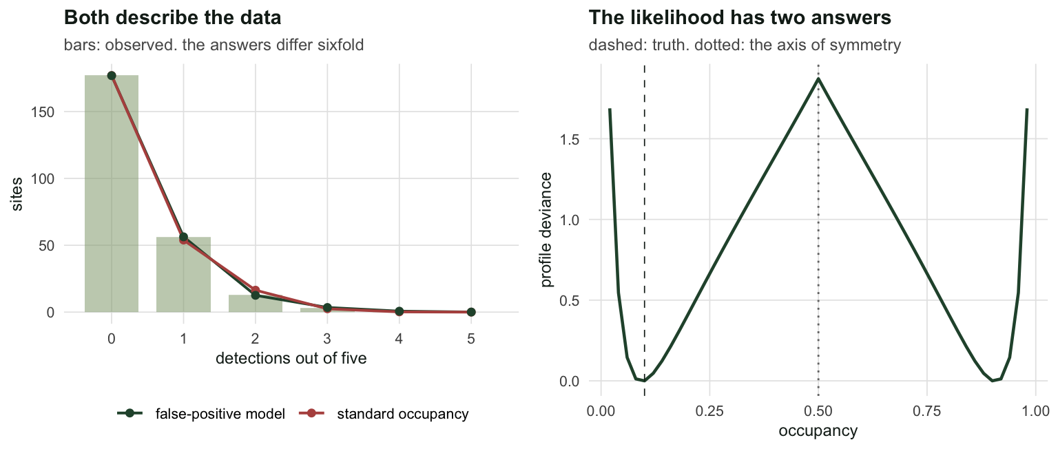
What picks the sensible one is not the likelihood but your prior conviction that a species is detected more reliably where it lives than where it does not, imposed as the constraint \(p_{11} > p_{10}\). That constraint is an assumption, and this model cannot test it. In a survey where a conspicuous look-alike, living mainly where a cryptic target is absent, is misrecorded as the target more often per visit than the target is recorded at its own sites, it is also the wrong assumption.
How bad, and when
One data set is an anecdote. Sweep the true occupancy across a range and refit, keeping everything else fixed. The false-positive model is fitted from one start in each well, and the better fit is reported with the labels that give \(p_{11} > p_{10}\).
psi_seq <- c(0.05, 0.10, 0.20, 0.30, 0.45, 0.60)
M <- 120L
sweep <- do.call(rbind, lapply(psi_seq, function(ps) {
  est <- t(sapply(1:M, function(m) {
    set.seed(70000L + m + round(ps * 1000))
    zz <- rbinom(R, 1L, ps)
    dd <- rowSums(matrix(rbinom(R * K, 1L,
      ifelse(rep(zz, K) == 1, p11_t, p10_t)), R, K))
    f_a <- fit_nm(fp_nll, c(0, qlogis(0.4), qlogis(0.05)), se = FALSE, d = dd, K = K)
    f_b <- fit_nm(fp_nll, c(0, qlogis(0.05), qlogis(0.4)), se = FALSE, d = dd, K = K)
    f_f <- if (f_b$nll < f_a$nll) f_b else f_a          # one start in each well
    c(occ = plogis(fit_nm(occ_nll, c(0, 0), se = FALSE, d = dd, K = K)$par[1]),
      fp = plogis(if (f_f$par[2] > f_f$par[3]) f_f$par[1] else -f_f$par[1]))  # label by p11 > p10
  }))
  data.frame(psi = ps, model = c("standard occupancy", "false-positive model"),
             bias = c(mean(est[, "occ"]) - ps, mean(est[, "fp"]) - ps))
}))
b_low <- sweep$bias[sweep$psi == 0.05 & sweep$model == "standard occupancy"]
b_high <- sweep$bias[sweep$psi == 0.60 & sweep$model == "standard occupancy"]
lv <- c("naive", "standard occupancy", "false-positive model")
df1 <- data.frame(what = factor(lv, levels = lv), est = c(naive, psi_occ, psi_fp))
df_ci <- data.frame(what = factor(lv[-1], levels = lv),
lo = c(ci_occ[1], ci_fp[1]), hi = c(ci_occ[2], ci_fp[2]))
p1 <- ggplot(df1, aes(est, what)) +
geom_vline(xintercept = psi_t, linetype = "dashed", colour = te_ink,
linewidth = 0.4) +
geom_errorbar(data = df_ci, aes(y = what, xmin = lo, xmax = hi),
inherit.aes = FALSE, orientation = "y", width = 0.12, colour = te_forest,
linewidth = 0.7) +
geom_point(size = 2.6, colour = te_rust) +
labs(title = "One in twenty visits was wrong", x = "estimated occupancy", y = NULL,
subtitle = "dashed: the truth, 0.10") +
theme_te()
p2 <- ggplot(sweep, aes(psi, bias, colour = model)) +
geom_hline(yintercept = 0, linetype = "dashed", colour = te_ink, linewidth = 0.3) +
geom_line(linewidth = 0.8) +
geom_point(size = 1.7) +
scale_colour_manual(values = c("standard occupancy" = te_rust,
"false-positive model" = te_forest)) +
labs(title = "The rarer the species, the worse", x = "true occupancy",
y = "mean bias in estimated occupancy",
subtitle = "120 replicates per point") +
theme_te()
two_panel(p1, p2)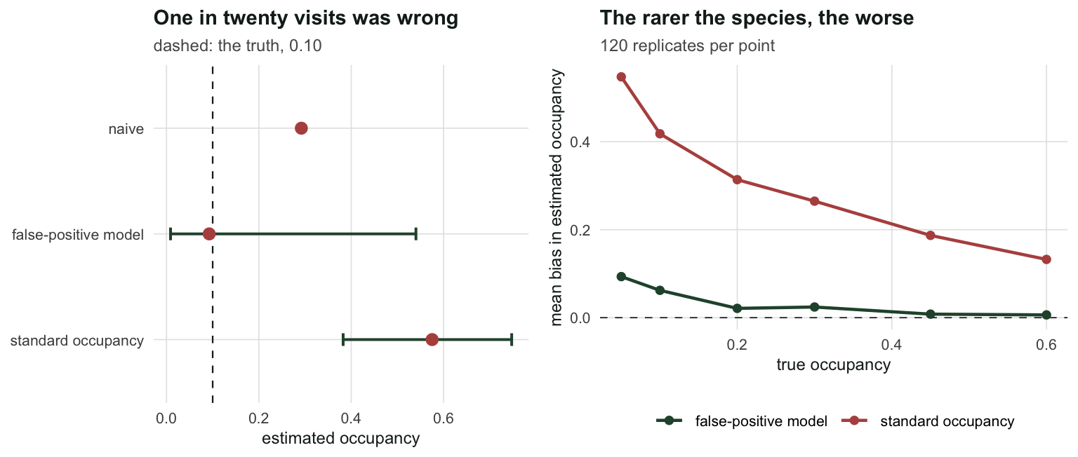
The bias runs from +0.547 at a true occupancy of 0.05 down to +0.132 at 0.60. This is the ugly part: the damage is worst exactly where occupancy models are most often used, which is on rare and cryptic species, and it shrinks as the species gets commoner but does not go away; at the right-hand end of the sweep the bias is still larger than the whole of the occupancy that the worked example above was trying to estimate. A 5% false-positive rate is not a small error in a landscape where the species occupies 5% of the sites. It is comparable to the signal.
What actually fixes it
The label swap says the detection data alone cannot pin down which mixture component is the species. So bring something else.
Miller et al. (2011) formalise the practical answer: make a subset of detections certain. Record two classes of observation, one that can be wrong, such as an acoustic identification, and one that cannot, such as a specimen in hand or a photograph a second observer confirms. Certain detections cannot arise at unoccupied sites, so any site with one is occupied, full stop, and that anchors the mixture.
set.seed(4275)
b_t <- 0.40
W <- matrix(0L, R, K)
for (i in 1:R) for (k in 1:K) {
  if (Y[i, k] == 1) {
    W[i, k] <- if (z[i] == 1 && rbinom(1, 1, b_t) == 1) 2L else 1L
  }
}
n1 <- rowSums(W == 1); n2 <- rowSums(W == 2); n0 <- K - n1 - n2

mil_nll <- function(par, n0, n1, n2, K) {
  psi <- plogis(par[1]); p11 <- plogis(par[2])
  p10 <- plogis(par[3]); b <- plogis(par[4])
  occ <- (1 - p11)^n0 * (p11 * (1 - b))^n1 * (p11 * b)^n2
  unocc <- ifelse(n2 > 0, 0, (1 - p10)^n0 * p10^n1)
  -sum(log(pmax(psi * occ + (1 - psi) * unocc, 1e-300)))
}
f_mil <- fit_nm(mil_nll, c(0, qlogis(0.4), qlogis(0.05), 0),
                n0 = n0, n1 = n1, n2 = n2, K = K)
psi_mil <- plogis(f_mil$par[1])
ci_mil <- plogis(f_mil$par[1] + c(-1.96, 1.96) * f_mil$se[1])
certain_sites <- sum(n2 > 0)
With 40% of true detections upgraded to certain, 12 sites are now known to be occupied without any modelling at all. The three-state model returns \(\hat\psi = 0.1132\) with an interval of [0.048, 0.242], against an interval 2.7 times as wide from the false-positive model, which had three parameters and no certain detections to work with on the same underlying sites.
That is the pattern worth taking away. The false-positive model does not extract more from the data; it declines to make a wrong assumption. What the estimator cannot supply is a class of observation which cannot lie, and only a field protocol produces that. The decision is made before anyone opens R. The Royle-Nichols model is the harder case: there, counts at a subset of sites sharpen the estimate only inside a detection model with a site effect, and the shape of that effect stays an assumption.
References
Link W 2003 Biometrics 59(4):1123-1130 (10.1111/j.0006-341X.2003.00129.x)
MacKenzie D, Nichols J, Lachman G, Droege S, Royle J, Langtimm C 2002 Ecology 83(8):2248-2255 (10.1890/0012-9658(2002)083[2248:ESORWD]2.0.CO;2)
Miller DA, Nichols JD, McClintock BT, Grant EHC, Bailey LL, Weir LA 2011 Ecology 92(7):1422-1428 (10.1890/10-1396.1)
Royle J, Link W 2006 Ecology 87(4):835-841 (10.1890/0012-9658(2006)87[835:GSOMAF]2.0.CO;2)