library(ggplot2)
library(grid)

te_ink <- "#16241d"; te_forest <- "#275139"; te_gold <- "#c9b458"
te_rust <- "#b5534e"; te_sage <- "#93a87f"

theme_te <- function() {
  theme_minimal(base_size = 11) +
    theme(
          plot.background  = element_rect(fill = "#f5f4ee", colour = NA),
          panel.background = element_rect(fill = "#f5f4ee", colour = NA),
          panel.grid.minor = element_blank(),
          panel.grid.major = element_line(colour = "grey90", linewidth = 0.3),
          plot.title = element_text(colour = te_ink, face = "bold", size = 11),
          plot.subtitle = element_text(colour = "grey35", size = 9),
          axis.title = element_text(colour = te_ink, size = 9),
          axis.text = element_text(colour = "grey30", size = 8),
          legend.position = "bottom",
          legend.title = element_blank(),
          legend.text = element_text(size = 8))
}
two_panel <- function(p1, p2) {
  grid.newpage()
  pushViewport(viewport(layout = grid.layout(1, 2)))
  print(p1, vp = viewport(layout.pos.row = 1, layout.pos.col = 1))
  print(p2, vp = viewport(layout.pos.row = 1, layout.pos.col = 2))
}Two-species occupancy and interactions
R
occupancy
imperfect detection
species interactions
ecology tutorial
Fitting the Rota multispecies occupancy model by hand in R, and watching a shared habitat gradient manufacture a species interaction that is not really there.
Two species, 400 sites, five visits each, two columns of ticks. Do they avoid each other?
The model that answers this question is not complicated, and it is well calibrated, and it will tell you with a z-statistic above 4 that two species interact when they do not. This post builds it, checks it properly, and then shows the single move that breaks it.
Four states instead of two
A single-species occupancy model has a latent state with two values: occupied or not. With two species the latent state has four: both present, only A, only B, neither. Rota et al. (2016) give each state a multinomial logit weight,
\[\Pr(z = 11) \propto e^{f_1 + f_2 + f_{12}}, \quad \Pr(z = 10) \propto e^{f_1}, \quad \Pr(z = 01) \propto e^{f_2}, \quad \Pr(z = 00) \propto 1,\]
so that \(f_1\) and \(f_2\) are the natural parameters for each species alone and \(f_{12}\) is the only term that couples them. Each species is then detected independently given its own presence, with probabilities \(p_A\) and \(p_B\).
The observation layer marginalises over whatever the four states could have been. A site where A was seen twice and B never could be state 11 with B missed five times, or state 10. A site where neither was seen could be any of the four. The likelihood adds up those possibilities.
state_probs <- function(f1, f2, f12) {
  num <- cbind(exp(f1 + f2 + f12), exp(f1), exp(f2), 1)
  num / rowSums(num)
}
rota_nll <- function(par, dA, dB, K, X = NULL) {
  n <- length(dA)
  if (is.null(X)) { f1 <- rep(par[1], n); f2 <- rep(par[2], n); f12 <- par[3]
    pA <- plogis(par[4]); pB <- plogis(par[5])
  } else { f1 <- par[1] + par[6] * X; f2 <- par[2] + par[7] * X; f12 <- par[3]
    pA <- plogis(par[4]); pB <- plogis(par[5])
  }
  P <- state_probs(f1, f2, f12)
  LA1 <- pA^dA * (1 - pA)^(K - dA); LA0 <- as.numeric(dA == 0)
  LB1 <- pB^dB * (1 - pB)^(K - dB); LB0 <- as.numeric(dB == 0)
  -sum(log(pmax(P[, 1] * LA1 * LB1 + P[, 2] * LA1 * LB0 +
                P[, 3] * LA0 * LB1 + P[, 4] * LA0 * LB0, 1e-300)))
}
ct <- list(maxit = 20000, reltol = 1e-12)
fit_rota <- function(dA, dB, K, X = NULL, start = NULL) {
  if (is.null(start)) start <- if (is.null(X)) rep(0, 5) else rep(0, 7)
  o <- optim(start, rota_nll, dA = dA, dB = dB, K = K, X = X,
             method = "Nelder-Mead", control = ct)
  o <- optim(o$par, rota_nll, dA = dA, dB = dB, K = K, X = X,
             method = "Nelder-Mead", control = ct)
  H <- optimHess(o$par, rota_nll, dA = dA, dB = dB, K = K, X = X)
  list(par = o$par, se = sqrt(diag(solve(H))), nll = o$value,
       aic = 2 * o$value + 2 * length(o$par))
}
gen <- function(R, f1, f2, f12, pA, pB, K, seed) {
  set.seed(seed)
  P <- state_probs(f1, f2, f12)
  s <- apply(P, 1, function(pr) sample.int(4, 1, prob = pr))
  zA <- as.integer(s %in% c(1, 2)); zB <- as.integer(s %in% c(1, 3))
  list(dA = rbinom(R, K, zA * pA), dB = rbinom(R, K, zB * pB), zA = zA, zB = zB)
}
Before fitting anything, one identity is worth checking, because it is what makes \(f_{12}\) interpretable at all. When \(f_{12} = 0\) the denominator factors, and
\[\Pr(z = 11) = \Pr(A) \Pr(B)\]
holds exactly, not approximately. The species interaction factor, \(\text{SIF} = \psi_{11} / (\psi_A \psi_B)\), is then exactly one.
sif <- function(f1, f2, f12) {
  P <- state_probs(f1, f2, f12)
  psiA <- P[1, 1] + P[1, 2]; psiB <- P[1, 1] + P[1, 3]
  P[1, 1] / (psiA * psiB)
}
sif_null <- sif(-0.2, -0.1, 0)
sif_pos <- sif(-0.2, -0.1, 1.2)
At \(f_{12} = 0\) the SIF is 1.000000000000, and at \(f_{12} = 1.2\) it is 1.1558. The parameter is a clean null: zero means independence in the latent state, whatever the detection probabilities happen to be.
It works
R <- 400L; K <- 5L
f1_t <- -0.2; f2_t <- -0.1; f12_t <- 1.2; pA_t <- 0.45; pB_t <- 0.40
g <- gen(R, rep(f1_t, R), rep(f2_t, R), f12_t, pA_t, pB_t, K, 4276)
fit <- fit_rota(g$dA, g$dB, K)
f12_ci <- fit$par[3] + c(-1.96, 1.96) * fit$se[3]
both_true <- sum(g$zA & g$zB)
both_seen <- sum(g$dA > 0 & g$dB > 0)
With \(f_{12} = 1.2\), the two species share 204 of 400 sites, but only 181 sites produced detections of both. The fit returns \(\hat{f}_{12} = 1.178\) with a standard error of 0.280, a 95% interval of [0.628, 1.727], and detection probabilities of 0.422 and 0.407 against truths of 0.45 and 0.40.
One fit proves nothing, so run it 200 times, and run it 200 more with the interaction switched off.
M <- 200L
mc_run <- function(f12, seed0) {
  t(sapply(1:M, function(m) {
    gg <- gen(R, rep(f1_t, R), rep(f2_t, R), f12, pA_t, pB_t, K, seed0 + m)
    ff <- fit_rota(gg$dA, gg$dB, K)
    c(est = ff$par[3], se = ff$se[3])
  }))
}
mc_alt <- mc_run(f12_t, 50000L)
mc_null <- mc_run(0, 60000L)
z_alt <- mc_alt[, "est"] / mc_alt[, "se"]
z_null <- mc_null[, "est"] / mc_null[, "se"]
cov95 <- mean(abs(mc_alt[, "est"] - f12_t) < 1.96 * mc_alt[, "se"])
power <- mean(abs(z_alt) > 1.96)
fpr <- mean(abs(z_null) > 1.96)
Over 200 replicates with a true interaction, the mean estimate is 1.234 against a truth of 1.2, a bias of +0.034. The Monte Carlo standard deviation is 0.268 and the mean reported standard error is 0.267, so the uncertainty the model reports is the uncertainty it has. Interval coverage is 0.945 and power to reject \(f_{12} = 0\) is 0.995. With no interaction, the test rejects 0.015 of the time.
The estimator is unbiased, its standard errors are honest, and its null test errs on the conservative side, rejecting less often than the nominal 0.05 rather than more. By every internal standard, this model works.
P_hat <- state_probs(fit$par[1], fit$par[2], fit$par[3])[1, ]
P_true <- state_probs(f1_t, f2_t, f12_t)[1, ]
lab <- c("both", "only A", "only B", "neither")
df1 <- data.frame(state = factor(rep(lab, 2), levels = lab),
                  prob = c(P_true, P_hat),
                  src = rep(c("true", "fitted"), each = 4))
p1 <- ggplot(df1, aes(state, prob, fill = src)) +
  geom_col(position = position_dodge(width = 0.7), width = 0.62) +
  scale_fill_manual(values = c("true" = te_sage, "fitted" = te_forest)) +
  labs(title = "The latent states are recovered", x = NULL, y = "probability",
       subtitle = "from ticks alone, no state is ever seen") +
  theme_te()

df2 <- data.frame(est = c(mc_null[, "est"], mc_alt[, "est"]),
                  scenario = rep(c("no interaction", "interaction of 1.2"), each = M))
p2 <- ggplot(df2, aes(est, fill = scenario)) +
  geom_histogram(bins = 26, alpha = 0.65, position = "identity") +
  geom_vline(xintercept = c(0, f12_t), linetype = "dashed", colour = te_ink,
             linewidth = 0.3) +
  scale_fill_manual(values = c("no interaction" = te_gold,
                               "interaction of 1.2" = te_forest)) +
  labs(title = "Calibrated and unbiased", x = "estimated interaction", y = "replicates",
       subtitle = "dashed: the two truths") +
  theme_te()
two_panel(p1, p2)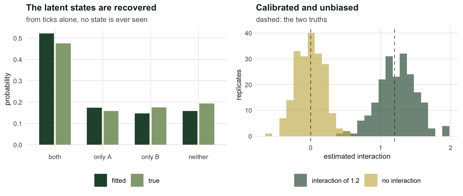
The move that breaks it
Now switch the interaction off entirely and give both species the same habitat preference. A gradient \(x\) runs across the sites; species A likes it, species B likes it, and neither has any opinion about the other. There is no interaction. There is nothing to find.
set.seed(4283)
x <- rnorm(R)
b1 <- 1.4; b2 <- 1.2; a1 <- -0.3; a2 <- -0.2
gc <- gen(R, a1 + b1 * x, a2 + b2 * x, 0, pA_t, pB_t, K, 4284)
fit_naive <- fit_rota(gc$dA, gc$dB, K)
fit_adj <- fit_rota(gc$dA, gc$dB, K, X = x)
ci_naive <- fit_naive$par[3] + c(-1.96, 1.96) * fit_naive$se[3]
ci_adj <- fit_adj$par[3] + c(-1.96, 1.96) * fit_adj$se[3]
z_naive <- fit_naive$par[3] / fit_naive$se[3]
z_adj <- fit_adj$par[3] / fit_adj$se[3]
Fitted without the covariate, the model reports \(\hat{f}_{12} = 1.151\), a 95% interval of [0.659, 1.643] that excludes zero comfortably, and \(z = 4.59\). That is the kind of number that ends up in an abstract.
Put \(x\) in the occupancy model and the interaction evaporates: \(\hat{f}_{12} = -0.114\), interval [-0.740, 0.512], \(z = -0.36\). The AIC prefers it by 186.6. Same sites, same ticks, same model, opposite conclusion.
None of this is a defect in the Rota model, which behaved impeccably in the previous section. Two species that both prefer wet ground will be found together more often than chance in exactly the way that mutual attraction predicts, and detection/non-detection data at a set of sites contain no information that separates those two stories. Blanchet et al. (2020) make the general argument at length: co-occurrence, however carefully modelled, is not evidence of interaction.
The obvious fix, and its price
“Measure the covariate” is the standard answer, and it works, and it is doing more assumption-shouldering than it looks. What you actually put in the model is a proxy: a soil moisture reading, a canopy index, an NDVI pixel. The gradient the species respond to is not the number in your column.
So repeat the adjusted fit, but corrupt \(x\) before handing it over.
sd_u <- c(0, 0.25, 0.5, 1.0, 2.0)
err <- t(sapply(sd_u, function(s) {
  set.seed(4290)
  w <- x + rnorm(R, 0, s)
  ff <- fit_rota(gc$dA, gc$dB, K, X = w)
  c(sd_u = s, est = ff$par[3], se = ff$se[3],
    rel = var(x) / (var(x) + s^2))
}))
err <- as.data.frame(err)
err$z <- err$est / err$se
df3 <- data.frame(
what = factor(c("no covariate", "covariate in model"),
levels = c("no covariate", "covariate in model")),
est = c(fit_naive$par[3], fit_adj$par[3]),
lo = c(ci_naive[1], ci_adj[1]), hi = c(ci_naive[2], ci_adj[2]))
p3 <- ggplot(df3, aes(est, what)) +
geom_vline(xintercept = 0, linetype = "dashed", colour = te_ink, linewidth = 0.4) +
geom_errorbar(aes(xmin = lo, xmax = hi), orientation = "y", width = 0.12, colour = te_forest,
linewidth = 0.7) +
geom_point(size = 2.6, colour = te_rust) +
labs(title = "There is no interaction in these data",
x = "estimated interaction", y = NULL,
subtitle = "dashed: the truth") +
theme_te()
p4 <- ggplot(err, aes(sd_u, est)) +
geom_hline(yintercept = 0, linetype = "dashed", colour = te_ink, linewidth = 0.3) +
geom_ribbon(aes(ymin = est - 1.96 * se, ymax = est + 1.96 * se),
fill = te_sage, alpha = 0.35) +
geom_line(linewidth = 0.8, colour = te_forest) +
geom_point(size = 1.8, colour = te_rust) +
labs(title = "The fix is only as good as the proxy",
x = "measurement error in the covariate",
y = "estimated interaction",
subtitle = "reliability falls from 1 to about 0.2 across this range") +
theme_te()
two_panel(p3, p4)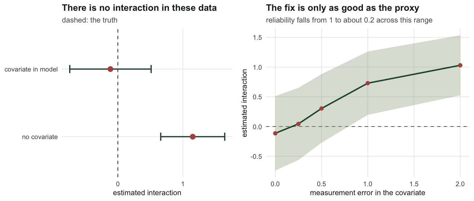
The spurious interaction comes back in proportion to the error. With a reliability of 0.51, meaning a covariate that is still correlated with the truth at 0.72, the estimate is back to 0.729 with \(z = 2.68\). A noisy covariate only partly adjusts, and the unadjusted remainder is deposited straight into \(f_{12}\), which is the only parameter left holding the residual association. This is regression dilution arriving in a place where nobody expects it, and the same arithmetic that governs confounding and backdoor adjustment governs it here.
What the parameter is
\(f_{12}\) is an association in the latent state after adjusting for whatever you put in the model. That is all it is. It is not a behavioural mechanism, not competition, and not exclusion, and calling it any of those is a claim about the world that the estimate cannot support.
Read that way, the model is still worth fitting. An association corrected for imperfect detection is a better description than an association not corrected for it, and Richmond et al. (2010) show how badly naive co-occurrence statistics mislead when detection differs between species. Just do not let the correction for one problem persuade you that the other problem went away with it. Whether the fit statistics can tell these worlds apart is taken up in checking an occupancy variant.
References
Blanchet F, Cazelles K, Gravel D 2020 Ecology Letters 23(7):1050-1063 (10.1111/ele.13525)
MacKenzie D, Nichols J, Lachman G, Droege S, Royle J, Langtimm C 2002 Ecology 83(8):2248-2255 (10.1890/0012-9658(2002)083[2248:ESORWD]2.0.CO;2)
Richmond O, Hines J, Beissinger S 2010 Ecological Applications 20(7):2036-2046 (10.1890/09-0470.1)
Rota C, Ferreira M, Kays R, Forrester T, Kalies E, McShea W, Parsons A, Millspaugh J 2016 Methods in Ecology and Evolution 7(10):1164-1173 (10.1111/2041-210X.12587)