library(ggplot2)
library(grid)

te_ink <- "#16241d"; te_forest <- "#275139"; te_gold <- "#c9b458"
te_rust <- "#b5534e"; te_sage <- "#93a87f"

theme_te <- function() {
  theme_minimal(base_size = 11) +
    theme(
          plot.background  = element_rect(fill = "#f5f4ee", colour = NA),
          panel.background = element_rect(fill = "#f5f4ee", colour = NA),
          panel.grid.minor = element_blank(),
          panel.grid.major = element_line(colour = "grey90", linewidth = 0.3),
          plot.title = element_text(colour = te_ink, face = "bold", size = 11),
          plot.subtitle = element_text(colour = "grey35", size = 9),
          axis.title = element_text(colour = te_ink, size = 9),
          axis.text = element_text(colour = "grey30", size = 8),
          legend.position = "bottom",
          legend.title = element_blank(),
          legend.text = element_text(size = 8))
}
two_panel <- function(p1, p2) {
  grid.newpage()
  pushViewport(viewport(layout = grid.layout(1, 2)))
  print(p1, vp = viewport(layout.pos.row = 1, layout.pos.col = 1))
  print(p2, vp = viewport(layout.pos.row = 1, layout.pos.col = 2))
}Checking an occupancy variant
R
occupancy
imperfect detection
model checking
ecology tutorial
Four latent stories, one set of detection frequencies. What goodness of fit and model selection can decide about occupancy models, and what they cannot.
Updated 25 September 2026: the abundance row of “So what does separate them” now follows the new calibration section of the Royle-Nichols post, where counts help only inside a detection model with a site effect.
The previous three posts each ended in the same place. The Royle-Nichols model reads unmodelled heterogeneity as abundance. The two-species model reads a shared habitat gradient as an interaction. The false-positive model cannot tell its answer from its own mirror image. In each case the escape route offered was mainly design, and in each case a reader is entitled to ask the obvious question first: can I not just check?
You can check. This post does the checking properly, with a calibrated test, and the answer is worse than you would like.
What the data actually are
Start with an observation that sounds like a computational footnote and is really the whole post.
With a detection probability that does not vary between visits, the order of the ticks carries no information. A site detected on visits 1 and 4 is exchangeable with a site detected on visits 2 and 5. All that survives is \(d_i\), the number of detections, and once you have that, all that survives is how many sites had each value of \(d\). With \(K\) visits, your 300 sites collapse to \(K+1\) numbers.
Nmax <- 80L; Nv <- 0:Nmax
p_occ <- function(th, K) { psi <- plogis(th[1]); p <- plogis(th[2])
  psi * dbinom(0:K, K, p) + c(1 - psi, rep(0, K)) }
p_rn <- function(th, K) { lam <- exp(th[1]); r <- plogis(th[2])
  colSums(dpois(Nv, lam) *
    t(sapply(Nv, function(n) dbinom(0:K, K, 1 - (1 - r)^n)))) }
p_mix <- function(th, K) { psi <- plogis(th[1]); p1 <- plogis(th[2])
  p2 <- plogis(th[3]); w <- plogis(th[4])
  psi * (w * dbinom(0:K, K, p1) + (1 - w) * dbinom(0:K, K, p2)) +
    c(1 - psi, rep(0, K)) }
p_fp <- function(th, K) { psi <- plogis(th[1]); p11 <- plogis(th[2])
  p10 <- plogis(th[3])
  psi * dbinom(0:K, K, p11) + (1 - psi) * dbinom(0:K, K, p10) }

pv <- list(occ = p_occ, rn = p_rn, mix = p_mix, fp = p_fp)
st <- list(occ = c(0, 0), rn = c(0, 0),
           mix = c(0, qlogis(0.4), qlogis(0.1), 0),
           fp = c(0, qlogis(0.4), qlogis(0.05)))
nl <- lapply(names(pv), function(k) {
  function(par, nvec, K) -sum(nvec * log(pmax(pv[[k]](par, K), 1e-300)))
})
names(nl) <- names(pv)
ct <- list(maxit = 8000, reltol = 1e-12)
fitn <- function(k, nvec, K) {
  o <- optim(st[[k]], nl[[k]], nvec = nvec, K = K, method = "Nelder-Mead",
             control = ct)
  o <- optim(o$par, nl[[k]], nvec = nvec, K = K, method = "Nelder-Mead",
             control = ct)
  list(par = o$par, nll = o$value, aic = 2 * o$value + 2 * length(st[[k]]))
}
tab <- function(d, K) as.numeric(table(factor(d, levels = 0:K)))

R <- 300L; K <- 6L
set.seed(4275); N <- rpois(R, 2.0); d_rn <- rbinom(R, K, 1 - (1 - 0.12)^N)
site_nll <- function(par, d, K) -sum(log(pmax(p_occ(par, K)[d + 1], 1e-300)))
chk <- abs(site_nll(c(0.3, -0.8), d_rn, K) - nl$occ(c(0.3, -0.8), tab(d_rn, K), K))
The site-by-site likelihood and the likelihood written on the frequency table agree to within floating-point rounding. They are the same function. The table is a sufficient statistic.
That reframes everything. The Royle-Nichols model has two parameters, the standard occupancy model has two, the false-positive model has three, and a two-point mixture has four. All four are competing explanations of the same 7 numbers, of which only 6 are free. They are all mixtures of binomials; they differ only in the shape of the mixing distribution and in which component gets called “occupied”. That is Link (2003) in a sentence, and it is why the rest of this post goes the way it does.
Four worlds
Build four data sets. Each has 300 sites and six visits and looks, to the eye, like ordinary detection/non-detection data.
set.seed(4273); z2 <- rbinom(R, 1L, 0.60); d_bet <- rbinom(R, K, z2 * rbeta(R, 1.2, 4.0))
set.seed(4276); z3 <- rbinom(R, 1L, 0.55); d_std <- rbinom(R, K, z3 * 0.30)
set.seed(4274); z4 <- rbinom(R, 1L, 0.10)
d_fp <- rowSums(matrix(rbinom(R * K, 1L,
  ifelse(rep(z4, K) == 1, 0.35, 0.05)), R, K))

worlds <- list(
  list(name = "abundance", d = d_rn, truth = 1 - exp(-2.0)),
  list(name = "heterogeneity", d = d_bet, truth = 0.60),
  list(name = "textbook", d = d_std, truth = 0.55),
  list(name = "false positives", d = d_fp, truth = 0.10))
The first was generated by the Royle-Nichols process: Poisson abundance with a mean of 2, each individual seen 12% of the time. The second has no abundance and Beta-distributed detection among occupied sites. The third is the textbook model, occupancy 0.55 and a constant detection probability of 0.30. The fourth has occupancy 0.10 and a 5% false-positive rate.
df_w <- do.call(rbind, lapply(worlds, function(w) {
  data.frame(d = 0:K, prop = tab(w$d, K) / R, world = w$name)
}))
df_w$world <- factor(df_w$world, levels = sapply(worlds, `[[`, "name"))
pw <- ggplot(df_w, aes(d, prop, colour = world)) +
  geom_line(linewidth = 0.7) +
  geom_point(size = 1.5) +
  scale_colour_manual(values = c(te_forest, te_rust, te_gold, te_sage)) +
  guides(colour = guide_legend(nrow = 2)) +
  scale_x_continuous(breaks = 0:K) +
  labs(title = "Four processes, four ordinary tables", x = "detections out of six",
       y = "proportion of sites",
       subtitle = "nothing here announces which model is right") +
  theme_te()

nv_rn <- tab(d_rn, K)
ks <- c("occ", "rn", "mix", "fp")
knm <- c("occupancy", "Royle-Nichols", "mixture", "false-positive")
df_f <- do.call(rbind, lapply(seq_along(ks), function(i) {
  data.frame(d = 0:K, count = R * pv[[ks[i]]](fitn(ks[i], nv_rn, K)$par, K),
             model = knm[i])
}))
pf <- ggplot() +
  geom_col(data = data.frame(d = 0:K, count = nv_rn), aes(d, count),
           fill = te_sage, alpha = 0.5, width = 0.75) +
  geom_line(data = df_f, aes(d, count, colour = model), linewidth = 0.6) +
  scale_colour_manual(values = c("occupancy" = te_rust,
                                 "Royle-Nichols" = te_forest,
                                 "mixture" = te_gold, "false-positive" = "grey55")) +
  guides(colour = guide_legend(nrow = 2)) +
  scale_x_continuous(breaks = 0:K) +
  labs(title = "Four models, one abundance world", x = "detections out of six",
       y = "sites", subtitle = "bars: observed. the curves nearly coincide") +
  theme_te()
two_panel(pw, pf)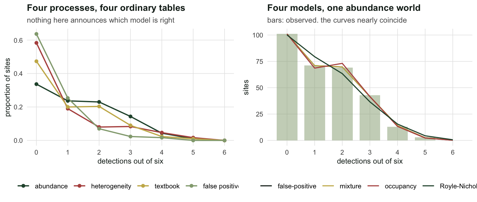
Fit the standard occupancy model to all four, and test it the way you are supposed to: the MacKenzie-Bailey goodness of fit, a Pearson chi-square on the detection frequencies with a parametric bootstrap null and an overdispersion factor.
X2f <- function(nvec, th, k, K) {
  e <- sum(nvec) * pv[[k]](th, K)
  sum((nvec - e)^2 / pmax(e, 1e-8))
}
gofn <- function(k, nvec, K, B, seed) {
  f <- fitn(k, nvec, K); obs <- X2f(nvec, f$par, k, K); Rn <- sum(nvec)
  set.seed(seed)
  bs <- replicate(B, {
    nb <- as.numeric(rmultinom(1, Rn, pv[[k]](f$par, K)))
    X2f(nb, fitn(k, nb, K)$par, k, K)
  })
  list(fit = f, p = mean(bs >= obs), chat = obs / mean(bs))
}
cal <- sapply(1:20, function(i) {
  set.seed(60000L + i); zz <- rbinom(R, 1L, 0.55); dd <- rbinom(R, K, zz * 0.30)
  gofn("occ", tab(dd, K), K, 150, 9275)$p
})
Before trusting the test, check that it is calibrated. On 20 data sets where the standard model is exactly true, the bootstrap p-values run from 0.04 to 0.94 with a mean of 0.476, and 1 of 20 below 0.05. The test is behaving.
res <- do.call(rbind, lapply(worlds, function(w) {
  nv <- tab(w$d, K); g <- gofn("occ", nv, K, 200, 9275); th <- g$fit$par
  se <- sqrt(diag(solve(optimHess(th, nl$occ, nvec = nv, K = K))))[1]
  sei <- se * sqrt(max(g$chat, 1))
  data.frame(world = w$name, truth = w$truth, naive = mean(w$d > 0),
             psi = plogis(th[1]), p = plogis(th[2]), gof = g$p, chat = g$chat,
             lo = plogis(th[1] - 1.96 * sei), hi = plogis(th[1] + 1.96 * sei))
}))
res$covers <- res$lo <= res$truth & res$truth <= res$hi
rn_row <- res[res$world == "abundance", ]| world | truth | fitted occupancy | GoF p | c-hat | corrected 95% interval |
|---|---|---|---|---|---|
| abundance | 0.865 | 0.753 | 0.925 | 0.181 | [0.681, 0.813] |
| heterogeneity | 0.600 | 0.467 | 0.005 | 6.356 | [0.311, 0.629] |
| textbook | 0.550 | 0.615 | 0.475 | 0.677 | [0.541, 0.684] |
| false positives | 0.100 | 0.574 | 0.015 | 6.340 | [0.279, 0.824] |
The test earns its keep in two rows and fails in the row that matters most.
On the heterogeneity data it fires: c-hat of 6.36, p of 0.005. On the false-positive data it fires: c-hat 6.34. Good. But on the abundance data, where the standard model is wrong about the process and reports an occupancy of 0.753 for a truth of 0.865, the goodness of fit returns p = 0.925 and an overdispersion factor of 0.181. That is not a marginal pass. It is the cleanest fit of the four worlds, cleaner than the world where the model is true.
And the c-hat correction cannot save it, because c-hat is below one: there is no overdispersion to correct. The interval stays narrow and stays wrong, missing the truth by 0.052 at its upper end.
Nothing is wrong with the residuals
This is worth pausing on, because it is not the usual failure. The fitted model reproduces the detection frequencies beautifully. It is not misfitting anything. The data really do look like 300 sites with an occupancy of 0.75 and a detection probability of 0.30, because a Poisson mixture of binomials with \(\lambda = 2\) and \(r = 0.12\) is very nearly a zero-inflated binomial with those parameters. The two mixing distributions produce almost the same 7 numbers.
The model is not failing to describe the data. It is describing the data correctly and calling the answer \(\psi\), when the thing it estimated is not \(\psi\). That is not something a residual can see.
Model selection does not adjudicate
If one model cannot check itself, try four and let the AIC decide.
aic_tab <- do.call(rbind, lapply(worlds, function(w) {
  nv <- tab(w$d, K)
  f <- lapply(c("occ", "rn", "mix", "fp"), fitn, nvec = nv, K = K)
  a <- sapply(f, `[[`, "aic")
  psis <- c(plogis(f[[1]]$par[1]), 1 - exp(-exp(f[[2]]$par[1])),
            plogis(f[[3]]$par[1]), plogis(f[[4]]$par[1]))
  data.frame(world = w$name, truth = w$truth,
             pick = c("occupancy", "Royle-Nichols", "mixture",
                      "false-positive")[which.min(a)],
             psi_pick = psis[which.min(a)],
             best = min(a), gap = sort(a)[2] - min(a))
}))| world | true occupancy | AIC picks | its occupancy | margin over runner-up |
|---|---|---|---|---|
| abundance | 0.865 | occupancy | 0.753 | 1.7 |
| heterogeneity | 0.600 | false-positive | 0.251 | 2.0 |
| textbook | 0.550 | occupancy | 0.615 | 2.0 |
| false positives | 0.100 | false-positive | 0.103 | 2.0 |
Look at the margins before the picks. Three of the four are almost exactly 2.0, and that number is not a coincidence.
nv_std <- tab(d_std, K)
f_o <- fitn("occ", nv_std, K); f_f <- fitn("fp", nv_std, K)
p10_fitted <- plogis(f_f$par[3])
nll_diff <- abs(f_o$nll - f_f$nll)
The false-positive model contains the standard occupancy model as the special case \(p_{10} = 0\). On the textbook data it finds exactly that: the fitted false-positive rate comes back as \(1.1 \times 10^{-11}\), and the two negative log-likelihoods differ by \(7.2 \times 10^{-11}\). The models fit identically. The AIC gap of 2.0000 is not a measurement of anything in the data; it is the parameter penalty and nothing else.
That is the situation across most of this table. These models are not rivals that the data can rank. They are nested or near-nested descriptions of the same 7 numbers, and the information criterion is left adjudicating on parameter count.
On the abundance data the AIC prefers the standard occupancy model over the Royle-Nichols model that generated it. On the heterogeneity data it picks the false-positive model, which reports an occupancy of 0.251 for a truth of 0.60, because a model with a spare mixture component will happily use it to describe heterogeneity that has nothing to do with misidentification. The false-positive model is not a false-positive detector. It is a two-component binomial mixture, and so is everything else on this list.
Not a seed
Everything above is one draw from each world, and a single draw can be unlucky. So repeat the abundance case 150 times: generate Royle-Nichols data, fit the standard model, run the goodness of fit, and record what a careful analyst would have concluded.
M <- 150L
psi_true <- 1 - exp(-2.0)
mc <- t(sapply(1:M, function(m) {
  set.seed(80000L + m); NN <- rpois(R, 2.0); dd <- rbinom(R, K, 1 - (1 - 0.12)^NN)
  nv <- tab(dd, K)
  g <- gofn("occ", nv, K, 100, 9275); th <- g$fit$par
  se <- sqrt(diag(solve(optimHess(th, nl$occ, nvec = nv, K = K))))[1]
  fits <- sapply(c("occ", "rn", "mix", "fp"), function(k) fitn(k, nv, K)$aic)
  c(psi = plogis(th[1]), gofp = g$p, chat = g$chat,
    cov_plain = as.numeric(abs(th[1] - qlogis(psi_true)) < 1.96 * se),
    cov_infl = as.numeric(abs(th[1] - qlogis(psi_true)) <
                          1.96 * se * sqrt(max(g$chat, 1))),
    pick = as.numeric(which.min(fits)))
}))
pass <- mean(mc[, "gofp"] > 0.05)
trap <- mean(mc[, "gofp"] > 0.05 & mc[, "cov_plain"] == 0)
Over 150 replicates the standard model’s occupancy estimate averages 0.7708 against a truth of 0.8647, a bias of -0.0938. The goodness of fit passes at the 5% level in 46.7% of the replicates, and c-hat comes out below one in 16.0% of them.
The nominal 95% interval covers the truth 18.0% of the time. Inflating it by the square root of c-hat, the standard remedy, lifts that to 52.0%. Neither is 95%. And in 38.7% of replicates the analyst gets a clean goodness of fit and an interval that excludes the truth, which is the worst of both worlds: a wrong answer with a certificate.
The AIC, given all four models, recovers the true Royle-Nichols model 69.3% of the time. The rest of the time it picks a model with a different biological meaning.
res$lab <- factor(res$world, levels = res$world)
p1 <- ggplot(res, aes(lab, chat, fill = chat > 1)) +
  geom_col(width = 0.62) +
  geom_hline(yintercept = 1, linetype = "dashed", colour = te_ink, linewidth = 0.4) +
  scale_fill_manual(values = c("FALSE" = te_sage, "TRUE" = te_rust),
                    labels = c("passes", "fires")) +
  labs(title = "The test misses the case that matters", x = NULL,
       y = "overdispersion factor",
       subtitle = "the standard model is wrong in three of these four") +
  theme_te() + theme(axis.text.x = element_text(angle = 20, hjust = 1))

df_mc <- data.frame(psi = mc[, "psi"],
                    gof = ifelse(mc[, "gofp"] > 0.05, "fit accepted",
                                 "fit rejected"))
p2 <- ggplot(df_mc, aes(psi, fill = gof)) +
  geom_histogram(bins = 24, alpha = 0.75, position = "stack") +
  geom_vline(xintercept = psi_true, linetype = "dashed", colour = te_ink,
             linewidth = 0.4) +
  scale_fill_manual(values = c("fit accepted" = te_gold,
                               "fit rejected" = te_forest)) +
  labs(title = "Half of these passed the check", x = "estimated occupancy",
       y = "replicates", subtitle = "dashed: the truth") +
  theme_te()
two_panel(p1, p2)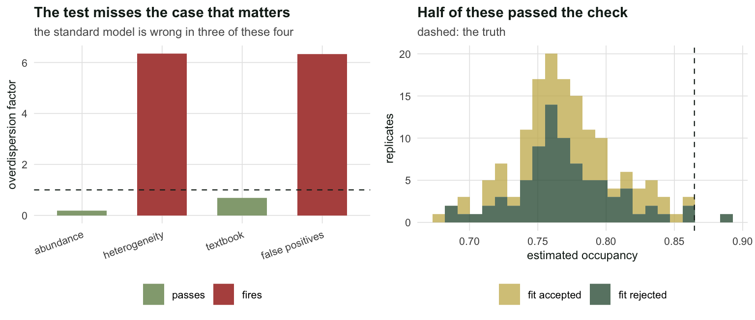
So what does separate them
Not the residuals, not the overdispersion factor, and not the information criterion. All three ask how well a model reproduces 6 numbers, and several models with incompatible biology reproduce them about equally well. The question they answer is not the question you asked.
What separates them is information from outside the detection table or, for abundance, an assumption stated out loud about the shape of the detection heterogeneity.
| to tell apart | you need | not |
|---|---|---|
| abundance from detection heterogeneity | a site effect in detection whose shape you are willing to assume, sharpened by counts or marks at some sites | counts fitted with a constant detection probability |
| interaction from shared habitat | the habitat covariate, measured well | a bigger model |
| false positives from low detection | a class of detection that cannot be wrong | a p10 parameter |
| any of them from the others | a design decision made in the field | any fit statistic |
Every row but the first is a decision taken before the data exist, and even the first leans on field data to sharpen it and on an assumption to anchor it. That is the uncomfortable part, and it is why the previous three posts all ended with protocol rather than a fit statistic.
None of this makes these models useless. A Royle-Nichols fit is a defensible estimate of abundance under an assumption you have stated out loud; the alternative of pretending detection is homogeneous is not more honest, only more familiar. The false-positive model is the right model when you have reason to believe in misidentification, and checking that an N-mixture model survives is subject to the same limits for the same reasons. What the checking machinery gives you is a genuine service: it catches the misfits it can catch, it is calibrated, and it will tell you when your model cannot even describe the frequencies. What it will never do is tell you which latent world produced them.
The deepest assumptions in an occupancy model, closure across visits, no unmodelled heterogeneity, and no false positives, are not hypotheses the data can weigh. They are the conditions under which the data mean what you think they mean.
References
Link W 2003 Biometrics 59(4):1123-1130 (10.1111/j.0006-341X.2003.00129.x)
MacKenzie D, Bailey L 2004 Journal of Agricultural, Biological, and Environmental Statistics 9(3):300-318 (10.1198/108571104X3361)
Royle J 2006 Biometrics 62(1):97-102 (10.1111/j.1541-0420.2005.00439.x)
Royle J, Link W 2006 Ecology 87(4):835-841 (10.1890/0012-9658(2006)87[835:GSOMAF]2.0.CO;2)
Royle J, Nichols J 2003 Ecology 84(3):777-790 (10.1890/0012-9658(2003)084[0777:EAFRPA]2.0.CO;2)
Kery M, Royle J 2016 Applied Hierarchical Modeling in Ecology. Academic Press (ISBN 978-0-12-801378-6)