Checking an N-mixture model

Diagnostics for a fitted N-mixture model in base R: a parametric-bootstrap fit test, site-level quantile residuals, and sensitivity to the abundance ceiling.

Corrected 7 October 2026: the post said the Freeman-Tukey statistic has no standard reference distribution because the mixture makes the counts more variable than a plain Poisson, and that site-total residuals are more informative because correlation from detection heterogeneity accumulates across visits; it now says that each count is Poisson under the model but the counts at a site share an abundance and so are correlated, and that the site totals give residuals that are independent of one another.

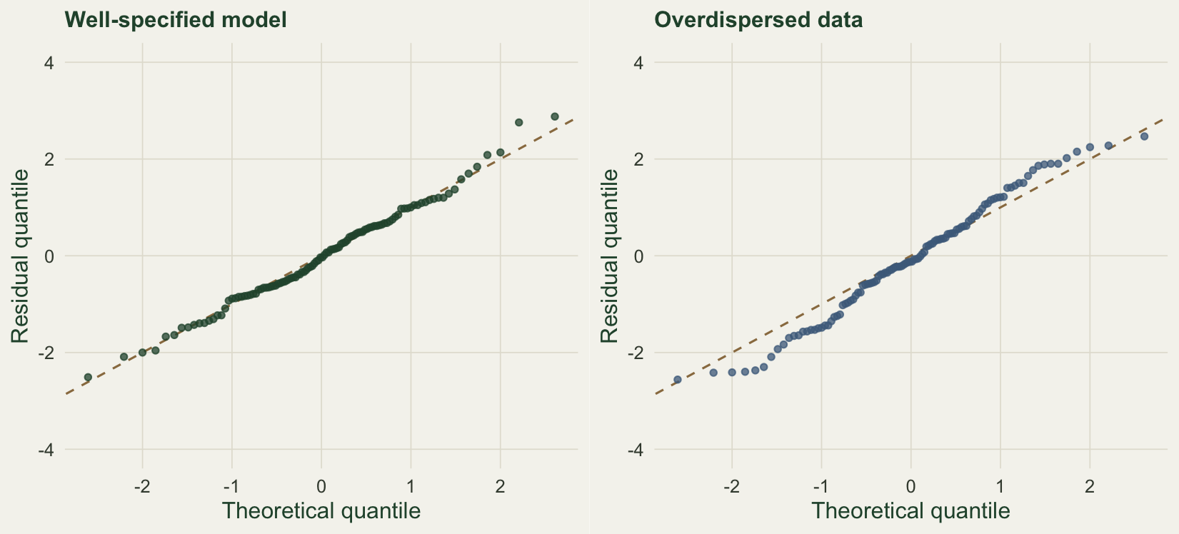
Corrected 1 October 2026: the post said the overdispersed residuals fan away from the line at the extremes, with heavier tails than a normal; in fact the points run steeper than the line while the most extreme residual at each end comes back to it, and the caption, alt text and text now say so.

The companion tutorial on N-mixture reliability showed how much can go wrong beneath a clean-looking abundance estimate: the fit can be unbounded, the negative-binomial dispersion can be unidentified, and unmodelled detection heterogeneity can inflate abundance without warning. The lesson is that a fitted N-mixture model has to be checked rather than trusted. This tutorial assembles the routine checks, coded from scratch: a parametric-bootstrap goodness-of-fit test that also returns an overdispersion ratio, quantile residuals that expose lack of fit, and a sensitivity check on the numerical ceiling. It closes on an honest limit, that these tests can pass while the abundance is still wrong.

The estimator is the marginal likelihood with the latent abundance summed out, in the same vectorised form used throughout this series:

library(ggplot2)

nll_pois <- function(par, y, K) {
  lam <- exp(par[1]); p <- plogis(par[2])
  Nv <- 0:K; lp <- dpois(Nv, lam, log = TRUE); ll <- 0
  for (i in seq_len(nrow(y))) {
    yi <- y[i, ]; idx <- (max(yi) + 1):(K + 1); Ni <- Nv[idx]
    lb <- rowSums(vapply(yi, function(v) dbinom(v, Ni, p, log = TRUE),
                         numeric(length(Ni))))
    ll <- ll + log(sum(exp(lp[idx] + lb)))
  }
  if (!is.finite(ll)) return(1e10)
  -ll
}
fit_pois <- function(y, K, start = c(log(2), 0))
  optim(start, nll_pois, y = y, K = K, method = "BFGS")

Goodness of fit by parametric bootstrap

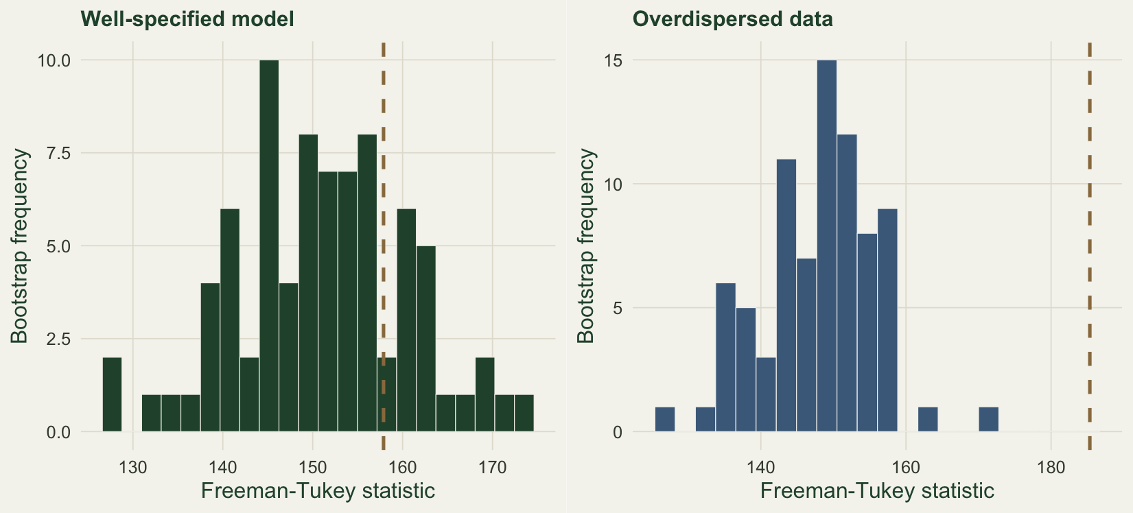
The natural fit statistic compares each observed count with what the fitted model expects. A single count has marginal mean equal to the product of abundance and detection, so a Freeman-Tukey discrepancy, which stabilises the variance of counts, sums the squared differences of square roots between observed and expected. Its value has no standard reference distribution here: each count on its own is Poisson under the model, but the counts at one site share an abundance and so are correlated, and the expected value is estimated from the same counts. The parametric bootstrap supplies the reference: simulate many data sets from the fitted model, refit each, and recompute the statistic, so the observed value is judged against the spread the model itself produces. The ratio of the observed statistic to the bootstrap mean is an overdispersion ratio, written c-hat: a value near one signals an adequate fit, and a value well above one flags variance the model has not captured (MacKenzie and Bailey 2004; Kery and Royle 2016).

# beta-binomial detection, used to build an overdispersed data set
rbb <- function(N, p, rho) {
  a <- p * (1 - rho) / rho; b <- (1 - p) * (1 - rho) / rho
  rbinom(length(N), N, rbeta(length(N), a, b))
}
ft <- function(y, lam, p) { E <- lam * p; sum((sqrt(y) - sqrt(E))^2) }

gof_boot <- function(y, K, B = 80, boot_seed = 1) {
  f <- fit_pois(y, K); lam <- exp(f$par[1]); p <- plogis(f$par[2])
  Tobs <- ft(y, lam, p); set.seed(boot_seed); Tb <- numeric(B)
  for (b in 1:B) {
    N  <- rpois(nrow(y), lam)
    ys <- matrix(rbinom(nrow(y) * ncol(y), rep(N, ncol(y)), p), nrow(y), ncol(y))
    fb <- fit_pois(ys, K); Tb[b] <- ft(ys, exp(fb$par[1]), plogis(fb$par[2]))
  }
  list(lam = lam, p = p, Tobs = Tobs, Tb = Tb,
       pval = mean(Tb >= Tobs), chat = Tobs / mean(Tb))
}

Tv <- 3L; K <- 40L; B <- 80L
set.seed(4280)                                   # a well-specified data set
R <- 110L; Ng <- rpois(R, 2.5)
yg <- matrix(rbinom(R * Tv, rep(Ng, Tv), 0.40), R, Tv)
set.seed(4261)                                   # detection heterogeneity added
Nb <- rpois(R, 2.5); yb <- sapply(1:Tv, function(t) rbb(Nb, 0.40, 0.30))

gg <- gof_boot(yg, K, B); gb <- gof_boot(yb, K, B)

For the well-specified data the observed statistic of 157.9 is judged against the bootstrap spread, giving a p-value of 0.237 and a c-hat of 1.05, and the abundance estimate is 2.51 against a truth of 2.5. For the overdispersed data the test rejects with a c-hat of 1.25: 0 of the 80 bootstrap statistics reach the observed one, a p-value of 0.012 once the observed statistic is counted among the draws. The same fit has quietly pushed abundance to 8.09, 3.2 times the truth, while reporting a detection probability of only 0.11.

Figure 1: Bootstrap distribution of the Freeman-Tukey statistic under the fitted model, with the observed value marked (dashed). For the well-specified data (left) the observed value falls within the range of the bootstrap draws. For the overdispersed data (right) it lies far into the upper tail.

Quantile residuals

A single test statistic reduces the whole fit to one number. Residuals show where it fails. For discrete data the right tool is the randomised-quantile residual (Dunn and Smyth 1996): evaluate the fitted cumulative distribution just below and at each observation, draw a uniform value between them, and map it through the normal quantile function, so a correct model yields residuals that are standard normal. Knape et al. (2018) show that residuals formed on the site totals are more informative for N-mixture models than per-count residuals, and with one total per site they are also independent of one another, which residuals of counts that share an abundance are not. The site total is convenient here: the sum of independent binomial counts that share an abundance is itself binomial in the total number of trials, so the total at a site with abundance N is Binomial with N times the number of visits as its size, and its marginal distribution follows by averaging over the Poisson abundance.

# marginal CDF of the site total S = sum of visits; S given N is Binomial(T*N, p)
Fss <- function(s, lam, p, Tv, K) { Nv <- 0:K; sum(dpois(Nv, lam) * pbinom(s, Tv * Nv, p)) }
rq_site <- function(y, lam, p, K, rseed = 99) {
  Tv <- ncol(y); S <- rowSums(y); set.seed(rseed)
  lo <- vapply(S, function(s) Fss(s - 1, lam, p, Tv, K), numeric(1))
  hi <- vapply(S, function(s) Fss(s,     lam, p, Tv, K), numeric(1))
  qnorm(pmin(pmax(runif(length(S), lo, hi), 1e-6), 1 - 1e-6))
}
rg <- rq_site(yg, gg$lam, gg$p, K); rb <- rq_site(yb, gb$lam, gb$p, K)

The residuals for the well-specified fit have a standard deviation of 1.03, close to one, with 6.4 per cent beyond the two-sigma band, near the expected five. The overdispersed fit spreads wider, a standard deviation of 1.22 and 10.9 per cent beyond two sigma, and in the quantile plot the points run steeper than the reference line, below it on the left and above it on the right, until the most extreme residual at each end comes back to it.

Figure 2: Normal quantile plots of site-level randomised-quantile residuals. Under the well-specified model (left) the points follow the reference line. Under the overdispersed model (right) the points run steeper than the line, below it on the left and above it on the right, although the most extreme residual at each end comes back to it: the residuals are too widely spread, the signature of variance the model has not absorbed.

Sensitivity to the ceiling

The reliability tutorial showed that when the fit is near unbounded, the abundance estimate climbs with the numerical ceiling K instead of settling. That makes ceiling sensitivity a fast, routine check: refit over a few values of K and confirm the estimate is stable.

set.seed(4254)                                   # low detection, unreliable
Rl <- 120L; Tl <- 2L; Nl <- rpois(Rl, 3.0)
yl <- matrix(rbinom(Rl * Tl, rep(Nl, Tl), 0.12), Rl, Tl)
Kseq <- c(30, 60, 120, 300)
lam_reliable   <- sapply(Kseq, function(K) exp(fit_pois(yg, K)$par[1]))
lam_unreliable <- sapply(Kseq, function(K) exp(fit_pois(yl, K, c(log(3), qlogis(0.2)))$par[1]))

The well-specified fit returns 2.51 at every ceiling from 30 to 300. The low-detection fit gives 14.3, 34, 78 and 226 as the ceiling rises. An estimate that moves with K is governed by an arbitrary bound rather than by the data, and should be discarded.

The honest limit: passing is necessary, not sufficient

A clean bill of health from these checks is reassuring but not conclusive. The bootstrap test catches gross overdispersion, as it did above with a c-hat of 1.25. It is far less sensitive to modest detection heterogeneity, which the reliability tutorial showed can still bias abundance. A mild version makes the point.

With mild heterogeneity the goodness-of-fit test does not reject here, a p-value of 0.725 and a c-hat of 0.98, yet abundance is estimated at 2.91, 17 per cent above the truth. The abundance estimate is more sensitive to the assumption than the fit statistics are, exactly the warning of Barker et al. (2018) and Link et al. (2018). Worse, overdispersion in detection and overdispersion in abundance are partly confounded (Knape et al. 2018), so a model that passes only after a negative-binomial term is added can still carry a biased abundance. The practical stance is the one the reliability tutorial reached: run these checks, report c-hat and residuals alongside the estimate, confirm stability in K, and treat a passing test as a floor rather than a guarantee. When an absolute abundance genuinely matters, identify detection directly with marked individuals rather than leaning on counts alone.

References

Knape, J., Arlt, D., Barraquand, F., Berg, A. and others 2018. Methods in Ecology and Evolution 9(10):2102-2114 (10.1111/2041-210X.13062).

Duarte, A., Adams, M.J. and Peterson, J.T. 2018. Ecological Modelling 374:51-59 (10.1016/j.ecolmodel.2018.02.007).

Dunn, P.K. and Smyth, G.K. 1996. Journal of Computational and Graphical Statistics 5(3):236-244 (10.1080/10618600.1996.10474708).

Barker, R.J., Schofield, M.R., Link, W.A. and Sauer, J.R. 2018. Biometrics 74(1):369-377 (10.1111/biom.12734).

Link, W.A., Schofield, M.R., Barker, R.J. and Sauer, J.R. 2018. Ecology 99(7):1547-1551 (10.1002/ecy.2362).

MacKenzie, D.I. and Bailey, L.L. 2004. Journal of Agricultural, Biological, and Environmental Statistics 9(3):300-318 (10.1198/108571104X3361).

Kery, M. and Royle, J.A. 2016. Applied Hierarchical Modeling in Ecology, Volume 1. Academic Press. ISBN 978-0-12-801378-6.

Related tutorials

• N-mixture reliability and the detection trade-off
• N-mixture models: abundance from repeated counts
• Checking an occupancy variant
• Checking a distance sampling model

Reproducibility

• Code last run: 2026-10-15
• R version 4.5.3 (2026-03-11), aarch64-apple-darwin20
• Packages: ggplot2 4.0.3