library(ggplot2)

nll_pois <- function(par, y, K) {           # Poisson-abundance marginal NLL
  lam <- exp(par[1]); p <- plogis(par[2])
  Nv <- 0:K; lp <- dpois(Nv, lam, log = TRUE); ll <- 0
  for (i in seq_len(nrow(y))) {
    yi <- y[i, ]; idx <- (max(yi) + 1):(K + 1); Ni <- Nv[idx]
    lb <- rowSums(vapply(yi, function(v) dbinom(v, Ni, p, log = TRUE),
                         numeric(length(Ni))))
    ll <- ll + log(sum(exp(lp[idx] + lb)))
  }
  if (!is.finite(ll)) return(1e10)
  -ll
}
fit_pois <- function(y, K, start = c(log(2), 0))
  optim(start, nll_pois, y = y, K = K, method = "BFGS",
control = list(reltol = 1e-12, maxit = 1000))N-mixture reliability and the detection trade-off
R
abundance
imperfect detection
model checking
ecology tutorial
When an N-mixture abundance estimate is unreliable: unbounded estimates, weakly identified dispersion, and inflation from unmodelled detection heterogeneity.
Corrected 8 October 2026: the post gave the stopping point of the negative-binomial fit as the value its dispersion lands at; the likelihood keeps rising towards the Poisson boundary, and the text now says the optimiser stops on the flat ridge on the way there. The inflation under the strongest detection heterogeneity is now given as an average over the replicate data sets rather than as a fixed figure.
Corrected 1 October 2026: the post said nothing in the counts announces unmodelled detection heterogeneity and that the model reports tight intervals around the inflated abundance; it now says the fit gives no warning of its own but the extra spread in the counts can be picked up by a goodness-of-fit check. The abundance fits also now run the optimiser to a tighter tolerance, which moves a few of the plotted estimates slightly.
Corrected 30 September 2026: the post said the median of the low-detection estimates sits near the truth, so the estimator is not biased; it now says the median is above the truth and forty surveys cannot settle the question of bias. It also said that Dennis, Morgan and Ridout give the exact condition for an infinite estimate; it now says they propose a diagnostic for one.
Corrected 27 September 2026: the post said that in 6 of the forty low-detection surveys the estimate follows the ceiling; three of those six settle from a ceiling of 120 upwards, so the count is now 3 and the figure colours only the lines that are still rising at the largest ceiling.
The binomial N-mixture model looks like a free lunch: point it at repeated counts, no marked animals, and it hands back abundance on an absolute scale. The catch is that the separation of abundance from detection rests entirely on the Poisson and constant-detection assumptions, and the counts alone carry almost no information to check them. When those assumptions bend, the estimate does not merely lose precision; it can run to infinity, hinge on a parameter the data cannot pin down, or double for reasons that have nothing to do with the population. This tutorial works through the three failures that matter most in practice, following the sceptical strand of the literature (Dennis, Morgan and Ridout 2015; Barker et al. 2018; Kery 2018; Link et al. 2018).
The estimator is the same marginal likelihood as before, with the latent abundance summed out. A vectorised version keeps the demonstrations quick:
Failure one: the estimate need not be finite
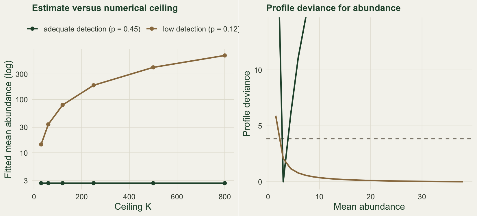
The marginal likelihood does not guarantee an interior maximum. When detection is low and counts are sparse, the likelihood is almost flat along the ridge where the product of abundance and detection matches the mean count, and it keeps improving, by a vanishing amount, as abundance rises and detection falls towards zero. There is then no finite maximum-likelihood estimate: the fitted abundance is pinned to whatever numerical ceiling K you impose, and raising the ceiling simply raises the answer. Dennis, Morgan and Ridout (2015) show that infinite estimates arise most readily when detection probability and the number of visits are small, and propose a sample covariance of the counts as a diagnostic, which performed well in the Poisson case; here we simply watch it occur.
set.seed(4254)
R <- 120L; Tv <- 2L                              # few visits, low detection
lam_true <- 3.0
Kgrid <- c(30, 120, 400, 800)
draw_lo <- function() {                          # one survey from the same design
  N <- rpois(R, lam_true)
  matrix(rbinom(R * Tv, rep(N, Tv), 0.12), R, Tv)
}
sets_lo <- replicate(40, draw_lo(), simplify = FALSE)
lam_lo  <- t(sapply(sets_lo, function(y)
  sapply(Kgrid, function(K) exp(fit_pois(y, K, c(log(3), qlogis(0.2)))$par[1]))))

set.seed(4255)                                   # contrast: adequate detection
N_ok   <- rpois(R, lam_true)
y_ok   <- matrix(rbinom(R * Tv, rep(N_ok, Tv), 0.45), R, Tv)
lam_ok <- sapply(Kgrid, function(K) exp(fit_pois(y_ok, K, c(log(3), 0))$par[1]))

base   <- lam_lo[, 1]                               # estimate at the lowest ceiling
tracks <- lam_lo[, ncol(lam_lo)] / lam_lo[, ncol(lam_lo) - 1] > 1.05  # still rising between the two largest ceilings
Forty surveys from the same design give forty different answers. Under adequate detection the ceiling does not matter: the fit is 2.69 at a ceiling of 30 and the same figure at 800. Under low detection the estimate at the lowest ceiling runs from 1.1 to 14.3 against a true mean of 3.0, a spread of more than tenfold between surveys that differ in nothing but the random draw. Their median, 3.74, is above the truth, and forty surveys this scattered cannot settle whether the estimator is biased; the clearer trouble is that one survey carries almost no information about abundance. And in 3 of the forty the estimate is not finite at all. It follows whatever ceiling is imposed, because the likelihood keeps improving, by a vanishing amount, as abundance rises and detection falls. An estimate that tracks the ceiling while the likelihood stays flat is an artefact of K, and the point estimate on its own will not tell you which of the two cases you are in.
Failure two: negative-binomial dispersion is barely identified
The Poisson assumption on abundance is often too rigid, and the natural fix is a negative-binomial mixture with an extra dispersion parameter. Kery (2018) screened well over a hundred bird data sets and found that Poisson and zero-inflated-Poisson N-mixtures were almost always identifiable, whereas negative-binomial versions frequently were not: the dispersion parameter drifts to its boundary and drags the abundance estimate with it. The mechanism is visible even on data that really are Poisson.
nll_nb <- function(par, y, K) {              # add a log-dispersion parameter
  lam <- exp(par[1]); p <- plogis(par[2]); sz <- exp(par[3])
  Nv <- 0:K; lp <- dnbinom(Nv, mu = lam, size = sz, log = TRUE); ll <- 0
  for (i in seq_len(nrow(y))) {
    yi <- y[i, ]; idx <- (max(yi) + 1):(K + 1); Ni <- Nv[idx]
    lb <- rowSums(vapply(yi, function(v) dbinom(v, Ni, p, log = TRUE),
                         numeric(length(Ni))))
    ll <- ll + log(sum(exp(lp[idx] + lb)))
  }
  if (!is.finite(ll)) return(1e10)
  -ll
}

set.seed(4256)
R <- 150L; Tv <- 3L; K <- 80L
N2 <- rpois(R, 2.8)
y2 <- matrix(rbinom(R * Tv, rep(N2, Tv), 0.35), R, Tv)   # genuinely Poisson
fp <- fit_pois(y2, K, c(log(2), 0))
fn <- optim(c(log(2), 0, log(5)), nll_nb, y = y2, K = K, method = "BFGS")
aic_p  <- 2 * fp$value + 2 * 2
aic_nb <- 2 * fn$value + 2 * 3
nb_size <- exp(fn$par[3])
# how flat is the dispersion? profile the negative log-likelihood at two sizes
prof_sz <- function(s) optim(c(log(2), 0),
  function(q) nll_nb(c(q[1], q[2], log(s)), y2, K), method = "Nelder-Mead")$value
nll_s100 <- prof_sz(100); nll_s1000 <- prof_sz(1000)
The negative-binomial fit adds a dispersion parameter to data that are Poisson by construction: its dispersion heads for the boundary where dispersion is infinite and the Poisson case sits, and the optimiser simply stops on the flat ridge on the way, here at 8472; its AIC is 1148.3 against the Poisson value of 1146.3. The dispersion is barely identified: increasing it tenfold, from 100 to 1000, changes the negative log-likelihood only from 571.28 to 571.17. On real data with genuine overdispersion the same flatness lets the estimate slide the other way, towards a small dispersion and a large abundance, which is exactly the instability Kery documents. The practical rule that follows is to prefer Poisson or zero-inflated-Poisson mixtures unless overdispersion is both clearly present and, as the next tutorial shows, actually checkable.
Failure three: unmodelled detection heterogeneity inflates abundance
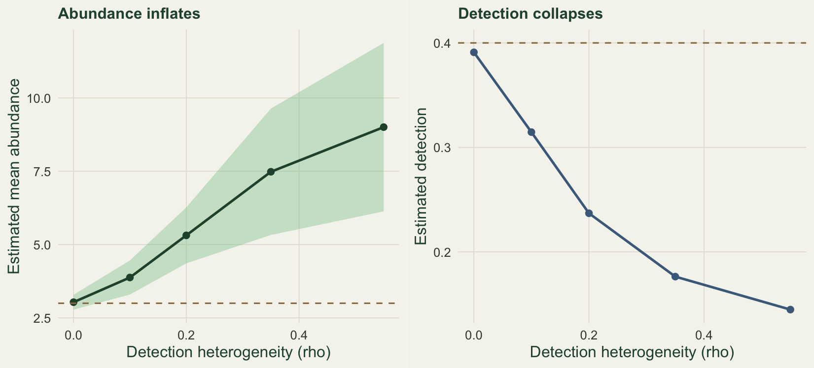
The most dangerous failure is the quietest. The model assumes every individual is detected with the same probability on a given visit, once covariates are accounted for. Real detection varies among individuals, visits and micro-sites in ways no covariate captures. Barker et al. (2018) and Link et al. (2018) showed that even small departures from constant detection can bias abundance badly, and that the counts give little warning. The reason is mechanical: extra variation in the counts looks, to the model, like extra variation in abundance, so it raises the mean abundance to explain the spread. We can watch the inflation grow by adding beta-binomial variation to detection and increasing it.
# beta-binomial counts: detection probability itself varies, with intra-visit
# correlation rho; rho = 0 is the ordinary binomial, larger rho is more heterogeneity
rbb <- function(N, p, rho) {
  a <- p * (1 - rho) / rho; b <- (1 - p) * (1 - rho) / rho
  rbinom(length(N), N, rbeta(length(N), a, b))
}
set.seed(4257)
R <- 150L; Tv <- 4L; K <- 55L; reps <- 8L; lam_true <- 3.0; p_true <- 0.40
rhos <- c(0.0001, 0.10, 0.20, 0.35, 0.55)
sweep <- do.call(rbind, lapply(rhos, function(rh) {
  m <- t(replicate(reps, {
    N <- rpois(R, lam_true); y <- sapply(1:Tv, function(t) rbb(N, p_true, rh))
    f <- fit_pois(y, K, c(log(3), qlogis(0.4))); c(exp(f$par[1]), plogis(f$par[2]))
  }))
  data.frame(rho = rh, lam = mean(m[, 1]), lam_sd = sd(m[, 1]), p = mean(m[, 2]))
}))
With no heterogeneity the fit is honest, recovering a mean abundance of 3.04 against the truth of 3.0. As detection heterogeneity rises, abundance inflates steadily, reaching 9.00 on average over the 8 data sets at the strongest level, roughly 200 per cent above the truth, while the estimated detection collapses from 0.39 towards 0.14. The fit itself gives no warning: its confidence interval comes from the same wrong model, so it can sit around a badly wrong number without reaching the truth, which is worse than an honestly wide one. The counts are not silent, though. Detection that varies like this spreads them more widely than a Poisson mixture with constant detection allows, and a check that looks for that extra spread, such as the bootstrap goodness-of-fit test and overdispersion ratio in the companion tutorial linked below, can pick it up, if less reliably when the heterogeneity is mild.
When the model can be trusted
None of this makes N-mixture models useless. It marks out where they are safe. A Poisson or zero-inflated-Poisson mixture, fitted to data with reasonably high detection and genuine population closure across visits, and checked for fit, gives defensible abundance. The trouble arrives with low detection, with negative-binomial dispersion added on faith, and above all with detection heterogeneity that no covariate removes. Barker et al. (2018) and Link et al. (2018) draw the blunt conclusion that when an absolute abundance really matters, the counts should be supplemented with data that identify detection directly, such as recaptures of marked individuals, rather than asked to do the job alone.
That leaves a practical question: given a single fitted model, how do you tell which regime you are in? The companion tutorial on checking an N-mixture model builds the diagnostics, from bootstrap goodness-of-fit and an overdispersion ratio to residual plots and the sensitivity to K we met above.
References
Dennis, E.B., Morgan, B.J.T. and Ridout, M.S. 2015. Biometrics 71(1):237-246 (10.1111/biom.12246).
Barker, R.J., Schofield, M.R., Link, W.A. and Sauer, J.R. 2018. Biometrics 74(1):369-377 (10.1111/biom.12734).
Kery, M. 2018. Ecology 99(2):281-288 (10.1002/ecy.2093).
Link, W.A., Schofield, M.R., Barker, R.J. and Sauer, J.R. 2018. Ecology 99(7):1547-1551 (10.1002/ecy.2362).
Royle, J.A. 2004. Biometrics 60(1):108-115 (10.1111/j.0006-341X.2004.00142.x).