library(ggplot2)
library(grid)

te_ink <- "#16241d"; te_forest <- "#275139"; te_gold <- "#c9b458"
te_rust <- "#b5534e"; te_sage <- "#93a87f"

theme_te <- function() {
  theme_minimal(base_size = 11) +
    theme(
          plot.background  = element_rect(fill = "#f5f4ee", colour = NA),
          panel.background = element_rect(fill = "#f5f4ee", colour = NA),
          panel.grid.minor = element_blank(),
          panel.grid.major = element_line(colour = "grey90", linewidth = 0.3),
          plot.title = element_text(colour = te_ink, face = "bold", size = 11),
          plot.subtitle = element_text(colour = "grey35", size = 9),
          axis.title = element_text(colour = te_ink, size = 9),
          axis.text = element_text(colour = "grey30", size = 8),
          legend.position = "bottom",
          legend.title = element_blank(),
          legend.text = element_text(size = 8))
}
two_panel <- function(p1, p2) {
  grid.newpage()
  pushViewport(viewport(layout = grid.layout(1, 2)))
  print(p1, vp = viewport(layout.pos.row = 1, layout.pos.col = 1))
  print(p2, vp = viewport(layout.pos.row = 1, layout.pos.col = 2))
}
The Royle-Nichols model: abundance from detections
R
occupancy
imperfect detection
abundance
ecology tutorial
How repeat visits let an occupancy model estimate abundance in R, why the trick works, and why unmodelled detection heterogeneity is read as abundance.
Corrected 15 October 2026: the random-effect fits in the test of counts integrated the site effect with too few quadrature nodes, which stopped some of them at spurious maxima; with an accurate rule more of the ticks-only fits run to the upper limit of the search, so abundance on ticks alone is even more weakly identified than the post said, and the conclusions stand.
Corrected 7 October 2026: the post said the Royle-Nichols model wins the model comparison on the data with no abundance; it now says it beats only the standard occupancy model, and that the two-point mixture fitted to the same ticks, with no abundance in it, has a lower AIC still.
Corrected 30 September 2026: the post said BFGS fails on the Royle-Nichols likelihood; on these data it finds the same maximum, and the failure described belongs to the standard occupancy fit. It also said one of the two ridge worlds leaves almost no sites without a detection, which mixed up empty sites with undetected ones.
Corrected 25 September 2026: the post said that counting animals at a subset of sites makes abundance identified by data. A new chunk tests that advice: the counts help only inside a detection model with a site effect, where they sharpen the estimate, and they do not repair a wrong assumption about the shape of that effect.
You visited 300 sites six times each and wrote down, for every visit, whether you saw the species. You never counted anything. The Royle-Nichols model claims it can tell you the mean number of individuals per site from those ticks alone.
That claim deserves suspicion, and this post spends most of its length earning it and then taking it back. The machinery works, the arithmetic is exact, and the estimate is nonetheless only as good as an assumption the data cannot check.
The idea in one line
A site with more individuals is easier to detect. If each of the \(N_i\) individuals at site \(i\) is seen independently on a visit with probability \(r\), then the site-level detection probability is not a constant but
\[p_i = 1 - (1 - r)^{N_i}.\]
Sites with \(N_i = 0\) have \(p_i = 0\): they are unoccupied. Sites with \(N_i = 5\) are far easier than sites with \(N_i = 1\). Put a Poisson prior on abundance, \(N_i \sim \text{Poisson}(\lambda)\), and marginalise it away:
\[\Pr(d_i \mid \lambda, r) = \sum_{N = 0}^{\infty} \frac{e^{-\lambda} \lambda^N}{N!} \binom{K}{d_i} \left[1 - (1-r)^N\right]^{d_i} \left[(1-r)^N\right]^{K - d_i},\]
where \(d_i\) is the number of visits out of \(K\) on which the species was recorded. Occupancy falls out as a derived quantity: a site is occupied when \(N_i > 0\), so \(\psi = 1 - e^{-\lambda}\).
That is the whole model (Royle and Nichols 2003). Two parameters, one infinite sum truncated in practice, and no marked individuals anywhere.
set.seed(4275)
R <- 300L; K <- 6L
lambda_true <- 2.0; r_true <- 0.12
N <- rpois(R, lambda_true)
d <- rbinom(R, K, 1 - (1 - r_true)^N)

Nmax <- 80L; Nv <- 0:Nmax
rn_nll <- function(par, d, K) {
  lam <- exp(par[1]); r <- plogis(par[2])
  pd <- colSums(dpois(Nv, lam) *
    t(sapply(Nv, function(n) dbinom(0:K, K, 1 - (1 - r)^n))))
  -sum(log(pmax(pd[d + 1], 1e-300)))
}
occ_nll <- function(par, d, K) {
  psi <- plogis(par[1]); p <- plogis(par[2])
  pd <- psi * dbinom(0:K, K, p) + c(1 - psi, rep(0, K))
  -sum(log(pmax(pd[d + 1], 1e-300)))
}
ct <- list(maxit = 8000, reltol = 1e-12)
fit_nm <- function(nll, start, d, K) {
  o <- optim(start, nll, d = d, K = K, method = "Nelder-Mead", control = ct)
  optim(o$par, nll, d = d, K = K, method = "Nelder-Mead", control = ct)
}
f_rn <- fit_nm(rn_nll, c(0, 0), d, K)
f_oc <- fit_nm(occ_nll, c(0, 0), d, K)

se_rn <- sqrt(diag(solve(optimHess(f_rn$par, rn_nll, d = d, K = K))))
lam_hat <- exp(f_rn$par[1]); r_hat <- plogis(f_rn$par[2])
lam_ci <- exp(f_rn$par[1] + c(-1.96, 1.96) * se_rn[1])
psi_rn <- 1 - exp(-lam_hat)
psi_oc <- plogis(f_oc$par[1])
psi_true <- 1 - exp(-lambda_true)
naive <- mean(d > 0)
The truth here is \(\lambda = 2.0\) individuals per site and \(r = 0.12\) per individual per visit, which puts true occupancy at \(\psi = 0.8647\). The species was recorded at least once at 66.3% of sites, so the naive estimate is already off by 0.20.
The fitted model returns \(\hat\lambda = 1.906\) with a 95% interval of [1.371, 2.648] and \(\hat{r} = 0.1333\), giving \(\hat\psi = 0.8513\) against a truth of 0.8647. A standard occupancy model on the same ticks reports \(\hat\psi = 0.7527\), which is 0.112 too low: with a single detection probability shared by all sites, the model has no way to know that the silent sites are silent because they are sparse rather than because they are empty.
A note on the optimiser, which matters more than it should. On these data BFGS on the log and logit scales, started from zero, reaches the same Royle-Nichols maximum as Nelder-Mead. The standard occupancy likelihood is less forgiving: BFGS from the same start runs off to an occupancy of one, reports success, and lands on a worse answer with a singular Hessian. Nelder-Mead restarted from its own solution, with optimHess for the standard errors, is slower and reaches the maximum in both cases.
Where the abundance actually comes from
Nothing in the data says “abundance”. The only thing the model sees is how often each site produced a detection. So which feature of those numbers carries the information?
Start with an exact identity. For \(N \sim \text{Poisson}(\lambda)\),
\[\mathbb{E}\left[(1-r)^N\right] = \sum_{N=0}^{\infty} \frac{e^{-\lambda}\lambda^N}{N!}(1-r)^N = e^{-\lambda r},\]
which is the probability of a non-detection on a single visit. With \(K = 1\) the likelihood depends on \(\lambda\) and \(r\) only through their product. Every pair with \(\lambda r = 0.24\) fits identically. The parameters are not merely imprecise, they are unidentified: the likelihood surface is an exact ridge.
prod_target <- lambda_true * r_true
lam_grid <- exp(seq(log(0.4), log(9), length.out = 60))
ridge <- data.frame(lambda = lam_grid, r = prod_target / lam_grid)
ridge <- ridge[ridge$r < 0.95, ]
nll_at <- function(lam, r, K, dd) rn_nll(c(log(lam), qlogis(r)), dd, K)

d1 <- rbinom(R, 1L, 1 - (1 - r_true)^N)
ridge$nll_k1 <- mapply(nll_at, ridge$lambda, ridge$r, MoreArgs = list(K = 1L, dd = d1))
ridge$nll_k6 <- mapply(nll_at, ridge$lambda, ridge$r, MoreArgs = list(K = K, dd = d))
spread_k1 <- diff(range(ridge$nll_k1))
spread_k6 <- diff(range(ridge$nll_k6))
Along that ridge the one-visit negative log-likelihood is constant: its values differ only by floating-point rounding. The six-visit likelihood varies by 288.86 over the same curve and has a clear minimum.
pair <- data.frame(lambda = c(1, 4), r = c(0.24, 0.06))
pair$empty <- dpois(0, pair$lambda)
pair$p_typ <- 1 - (1 - pair$r)^round(pair$lambda)
pair$p_one <- 1 - exp(-pair$lambda * pair$r)
pair$zero6 <- exp(-pair$lambda * (1 - (1 - pair$r)^K))  # no detection in K visits
The repeat visits are what break the tie, and it is worth seeing why. Take two points on the ridge. With \(\lambda = 1\) and \(r = 0.24\), 36.8% of sites hold nothing and are silent forever, while a typical occupied site is detected about 24% of the time. With \(\lambda = 4\) and \(r = 0.06\), only 1.8% of sites are empty, and a typical site is detected about 22% of the time. Both worlds produce a detection on 21.3% of single visits, which is why one visit cannot separate them. Six visits can, because the two worlds spread their detections differently: after six visits the first leaves 44.6% of sites with no detection at all and the second 28.9%, and the first has more sites detected on three or more visits, since its occupied sites are fewer but easier to detect. Abundance is inferred from the shape of the detection-frequency table, not from any count.
obs <- as.numeric(table(factor(d, levels = 0:K)))
exp_occ <- R * (plogis(f_oc$par[1]) * dbinom(0:K, K, plogis(f_oc$par[2])) +
                c(1 - plogis(f_oc$par[1]), rep(0, K)))
exp_rn <- R * colSums(dpois(Nv, lam_hat) *
  t(sapply(Nv, function(n) dbinom(0:K, K, 1 - (1 - r_hat)^n))))

df1 <- data.frame(d = rep(0:K, 2), count = c(exp_occ, exp_rn),
                  model = rep(c("standard occupancy", "Royle-Nichols"), each = K + 1))
p1 <- ggplot() +
  geom_col(data = data.frame(d = 0:K, count = obs), aes(d, count),
           fill = te_sage, alpha = 0.55, width = 0.75) +
  geom_line(data = df1, aes(d, count, colour = model), linewidth = 0.7) +
  geom_point(data = df1, aes(d, count, colour = model), size = 1.6) +
  scale_colour_manual(values = c("standard occupancy" = te_rust,
                                 "Royle-Nichols" = te_forest)) +
  scale_x_continuous(breaks = 0:K) +
  labs(title = "Observed and fitted detection frequencies", x = "detections out of six",
       y = "sites", subtitle = "bars: observed") +
  theme_te()

df2 <- data.frame(lambda = rep(ridge$lambda, 2),
                  nll = c(ridge$nll_k1 - min(ridge$nll_k1),
                          ridge$nll_k6 - min(ridge$nll_k6)),
                  visits = rep(c("one visit", "six visits"), each = nrow(ridge)))
p2 <- ggplot(df2, aes(lambda, nll, colour = visits)) +
  geom_line(linewidth = 0.8) +
  geom_vline(xintercept = lambda_true, linetype = "dashed",
             colour = te_ink, linewidth = 0.3) +
  scale_colour_manual(values = c("one visit" = te_gold, "six visits" = te_forest)) +
  scale_x_log10() +
  labs(title = "Negative log-likelihood along the ridge",
       x = "abundance (log scale)",
       y = "negative log-likelihood, relative",
       subtitle = "along the curve where abundance times detection is fixed") +
  theme_te()
two_panel(p1, p2)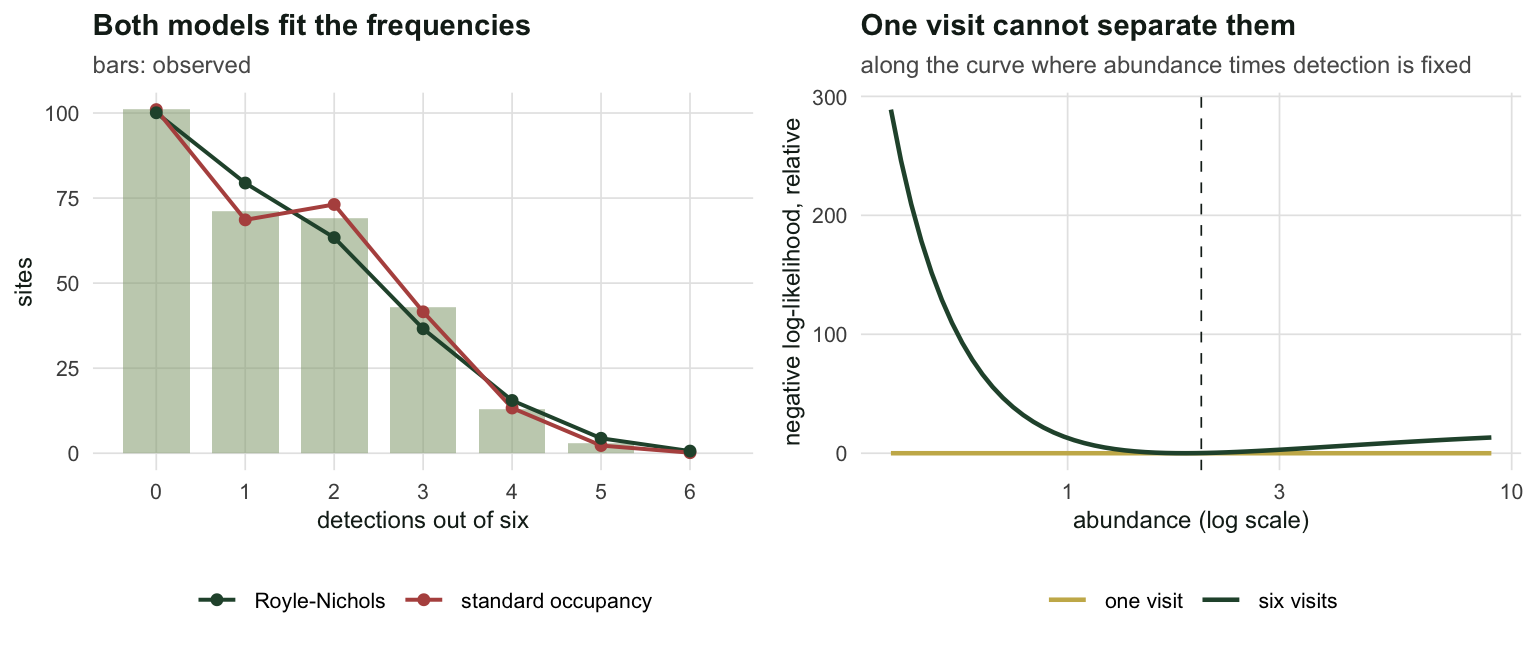
The part that should worry you
Here is the problem. Abundance is not the only thing that makes some sites easier than others. Wind, canopy, observer skill, time of day, and the animal’s own behaviour all produce sites where detection is high and sites where it is low. The Royle-Nichols model has one slot for site-level variation in detection, and that slot is labelled abundance. Anything that lands in it comes out wearing that label.
So simulate a world with no abundance at all. Every occupied site holds the species and nothing else is known about it; detection probability varies across occupied sites according to a Beta distribution. There is no \(N\), no \(\lambda\), no counting to be done.
set.seed(4273)
z_het <- rbinom(R, 1L, 0.60)
p_het <- rbeta(R, 1.2, 4.0)
d_het <- rbinom(R, K, z_het * p_het)

mix_nll <- function(par, d, K) {
  psi <- plogis(par[1]); p1 <- plogis(par[2]); p2 <- plogis(par[3]); w <- plogis(par[4])
  pd <- psi * (w * dbinom(0:K, K, p1) + (1 - w) * dbinom(0:K, K, p2)) +
        c(1 - psi, rep(0, K))
  -sum(log(pmax(pd[d + 1], 1e-300)))
}
aic <- function(f, k) 2 * f$value + 2 * k
h_oc <- fit_nm(occ_nll, c(0, 0), d_het, K)
h_rn <- fit_nm(rn_nll, c(0, 0), d_het, K)
h_mx <- fit_nm(mix_nll, c(0, qlogis(0.4), qlogis(0.1), 0), d_het, K)
lam_het <- exp(h_rn$par[1])
se_het <- sqrt(diag(solve(optimHess(h_rn$par, rn_nll, d = d_het, K = K))))
lam_het_ci <- exp(h_rn$par[1] + c(-1.96, 1.96) * se_het[1])
Fitted to data containing no individuals to count, the Royle-Nichols model reports \(\hat\lambda = 0.705\) individuals per site, with a 95% interval of [0.563, 0.882] that excludes nothing of interest and certainly does not warn you. Worse, it beats the standard occupancy model: AIC 768.5 against 779.4. Against a model with one detection probability for every site, model selection rewards the model that invented a quantity out of nothing, because that quantity is a perfectly good description of heterogeneity, which is really there. Only its name is wrong. A two-point mixture with no abundance in it, fitted to the same ticks and drawn in the left panel of the figure below, does better still at an AIC of 759.8: what model selection rewards here is the heterogeneity, not the abundance.
The mirror image is worse still. Return to the genuine Royle-Nichols data, where abundance really does drive detection, and fit a two-point finite mixture instead: occupied sites are either easy or hard, in some proportion, with no abundance anywhere in the specification.
g_mx <- fit_nm(mix_nll, c(0, qlogis(0.4), qlogis(0.1), 0), d, K)
psi_mx <- plogis(g_mx$par[1])
aic_rn <- aic(f_rn, 2); aic_mx <- aic(g_mx, 4)

prof_psi <- function(psi_fix, d, K) {
  f <- function(q) {
    p1 <- plogis(q[1]); p2 <- plogis(q[2]); w <- plogis(q[3])
    pd <- psi_fix * (w * dbinom(0:K, K, p1) + (1 - w) * dbinom(0:K, K, p2)) +
          c(1 - psi_fix, rep(0, K))
    -sum(log(pmax(pd[d + 1], 1e-300)))
  }
  o <- optim(c(qlogis(0.4), qlogis(0.1), 0), f, method = "Nelder-Mead", control = ct)
  optim(o$par, f, method = "Nelder-Mead", control = ct)$value
}
prof_rn <- function(psi_fix, d, K) {
  lam_fix <- -log(1 - psi_fix)
  f <- function(q) rn_nll(c(log(lam_fix), q), d, K)
  optimise(f, c(-8, 4))$objective
}
psi_grid <- seq(0.70, 0.999, length.out = 26)
dev_mx <- 2 * (sapply(psi_grid, prof_psi, d = d, K = K) - g_mx$value)
dev_rn <- 2 * (sapply(psi_grid, prof_rn, d = d, K = K) - f_rn$value)
dev_mx_at_truth <- 2 * (prof_psi(psi_true, d, K) - g_mx$value)
On the same detection histories the mixture reports \(\hat\psi = 1.000\), against the Royle-Nichols answer of 0.851 and a truth of 0.865. The AIC gap between them is 0.1. And the mixture’s answer is not an optimiser failure: its profile deviance is monotone up to the boundary, sitting at 0.01 when \(\psi\) is pinned at the true value, against the 3.84 cutoff.
obs_h <- as.numeric(table(factor(d_het, levels = 0:K)))
ex <- function(par, kind) {
  if (kind == "occ") R * (plogis(par[1]) * dbinom(0:K, K, plogis(par[2])) +
                          c(1 - plogis(par[1]), rep(0, K)))
  else if (kind == "rn") R * colSums(dpois(Nv, exp(par[1])) *
      t(sapply(Nv, function(n) dbinom(0:K, K, 1 - (1 - plogis(par[2]))^n))))
  else R * (plogis(par[1]) * (plogis(par[4]) * dbinom(0:K, K, plogis(par[2])) +
      (1 - plogis(par[4])) * dbinom(0:K, K, plogis(par[3]))) +
      c(1 - plogis(par[1]), rep(0, K)))
}
df3 <- data.frame(d = rep(0:K, 3),
                  count = c(ex(h_oc$par, "occ"), ex(h_rn$par, "rn"), ex(h_mx$par, "mix")),
                  model = rep(c("standard occupancy", "Royle-Nichols", "two-point mixture"),
                              each = K + 1))
p3 <- ggplot() +
  geom_col(data = data.frame(d = 0:K, count = obs_h), aes(d, count),
           fill = te_sage, alpha = 0.55, width = 0.75) +
  geom_line(data = df3, aes(d, count, colour = model), linewidth = 0.7) +
  scale_colour_manual(values = c("standard occupancy" = te_rust,
                                 "Royle-Nichols" = te_forest,
                                 "two-point mixture" = te_gold)) +
  guides(colour = guide_legend(nrow = 2)) +
  scale_x_continuous(breaks = 0:K) +
  labs(title = "Observed and fitted detection frequencies",
       x = "detections out of six", y = "sites",
       subtitle = "bars: observed, from the simulation with no abundance") +
  theme_te()

df4 <- data.frame(psi = rep(psi_grid, 2), dev = c(dev_rn, dev_mx),
                  model = rep(c("Royle-Nichols", "two-point mixture"),
                              each = length(psi_grid)))
p4 <- ggplot(df4, aes(psi, dev, colour = model)) +
  geom_line(linewidth = 0.8) +
  geom_hline(yintercept = qchisq(0.95, 1), linetype = "dotted", colour = "grey40") +
  geom_vline(xintercept = psi_true, linetype = "dashed", colour = te_ink,
             linewidth = 0.3) +
  scale_colour_manual(values = c("Royle-Nichols" = te_forest,
                                 "two-point mixture" = te_gold)) +
  coord_cartesian(ylim = c(0, 12)) +
  labs(title = "Profile deviance for occupancy",
       x = "occupancy", y = "profile deviance",
       subtitle = "dashed: truth. dotted: the 3.84 cutoff") +
  theme_te()
two_panel(p3, p4)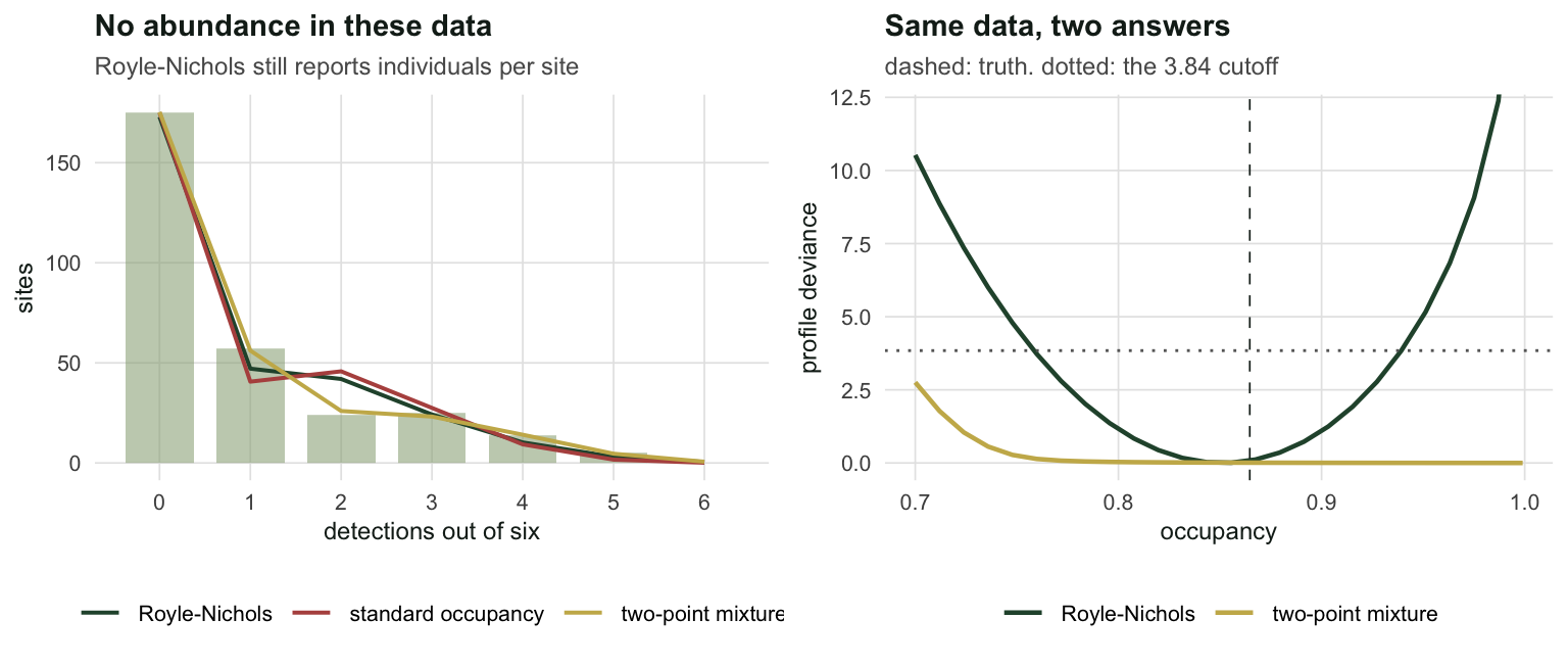
What this means when you have real ticks
The two failures are the same failure seen from opposite sides. Site-level variation in detection is real and estimable; its cause is not. Royle (2006) makes the point directly for occupancy models, and Link (2003) proved the general version for closed-population abundance: different mixing distributions can produce near-identical data and quite different inferences, and no quantity of data resolves the choice, because the choice is not in the data.
So the honest reading of a Royle-Nichols fit is narrow. The \(\hat\lambda\) is an estimate of mean abundance if you are willing to assert that abundance is the only source of site-level heterogeneity in detection, that individuals are detected independently, and that the abundance distribution is Poisson. The first of those three is an ecological claim about your field protocol, not a statistical one, and it is exactly the claim that fails when you survey along a gradient of vegetation density.
Model selection cannot settle the question either. On the very data set generated above, the standard occupancy model has an AIC of 908.6 against the Royle-Nichols model’s 912.3, and, whichever way that comparison falls, it is wrong about occupancy by 0.112. What the fit statistics can and cannot decide here is the subject of checking an occupancy variant, and it is not a comfortable read.
The design advice usually given at this point is to count something, even crudely, at a subset of sites, so that abundance is identified by data rather than by assumption. That advice can be tested. The next chunk builds a world in which detection varies between sites for a reason that has nothing to do with abundance: every site gets its own per-individual detection probability, logit-normal with a median of 0.15 and a standard deviation of 1 on the logit scale, fixed across the 5 visits, while abundance is Poisson with mean 1.5 at each of 200 sites. At 40 of those sites the observer writes down the count on every visit; the rest give only ticks. Each simulated data set is fitted four ways. The Royle-Nichols model uses the ticks from all 200 sites; the calibrated version uses the ticks from the uncounted sites and adds the counts through an N-mixture likelihood. Each of the two is fitted once with a single per-individual detection probability and once with a logit-normal site effect on it, which is the heterogeneous-detection model of Royle (2006) with an abundance layer underneath, integrated by Gauss-Hermite quadrature. A second batch repeats the fits when the true site effect is two-point (a site is either easy or hard, at plus or minus 1 on the logit scale), so that the fitted logit-normal family is wrong.
set.seed(6512)
cal_R <- 200L; cal_K <- 5L; cal_lam <- 1.5; cal_r0 <- 0.15; cal_sd <- 1
cal_m <- 40L; cal_Nv <- 0:60
gh_nodes <- function(n) {  # Gauss-Hermite nodes and log weights for a N(0, 1) effect
  i <- 1:(n - 1); b <- sqrt(i / 2); J <- matrix(0, n, n)
  J[cbind(i, i + 1)] <- b; J[cbind(i + 1, i)] <- b
  e <- eigen(J, symmetric = TRUE)
  list(x = e$values * sqrt(2), lw = log(e$vectors[1, ]^2))
}
gh <- gh_nodes(40)  # 15 nodes left spurious maxima on the flat abundance ridge; 80 change no number below
lse_rows <- function(M) {
  mx <- M[cbind(seq_len(nrow(M)), max.col(M, "first"))]
  mx + log(rowSums(exp(M - mx)))
}
sim_cal <- function(family) {
  N_site <- rpois(cal_R, cal_lam)
  z <- if (family == "logit-normal") rnorm(cal_R) else sample(c(-1, 1), cal_R, replace = TRUE)
  r_site <- plogis(qlogis(cal_r0) + cal_sd * z)  # per-individual detection, fixed per site
  y <- matrix(rbinom(cal_R * cal_K, rep(N_site, cal_K), rep(r_site, cal_K)), cal_R)
  ticks <- rowSums(y > 0); cnt <- y[seq_len(cal_m), ]  # counts kept at the first 40 sites
  list(tab_all = tabulate(ticks + 1, cal_K + 1),
       tab_rest = tabulate(ticks[-seq_len(cal_m)] + 1, cal_K + 1),
       cconst = sapply(cal_Nv, function(n) rowSums(lchoose(n, cnt))), Sy = rowSums(cnt))
}
pd_rn <- function(lpN, r) {  # P(d = 0..K detections) under Royle-Nichols with one r
  q <- 1 - (1 - r)^cal_Nv
  as.vector(outer(0:cal_K, q, function(k, qq) dbinom(k, cal_K, qq)) %*% exp(lpN))
}
cal_nll <- function(par, dat, arm) {
  lpN <- dpois(cal_Nv, exp(par[1]), log = TRUE)
  re <- arm %in% c("rn_re", "nm_re")
  rv <- if (re) plogis(par[2] + exp(par[3]) * gh$x) else plogis(par[2])
  Lrn <- sapply(rv, function(r) log(pmax(pd_rn(lpN, r), 1e-300)))
  tab <- if (arm %in% c("rn", "rn_re")) dat$tab_all else dat$tab_rest
  s <- if (re) sum(tab * lse_rows(Lrn + rep(gh$lw, each = cal_K + 1))) else sum(tab * Lrn)
  if (arm %in% c("nm", "nm_re")) {  # N-mixture likelihood of the counts at the counted sites
    Lc <- log(exp(dat$cconst + rep(lpN, each = cal_m)) %*% outer(cal_K * cal_Nv, log(1 - rv),
      function(a, b) exp(a * b))) + outer(dat$Sy, qlogis(rv))  # sites x nodes
    s <- s + if (re) sum(lse_rows(Lc + rep(gh$lw, each = cal_m))) else sum(Lc)
  }
  -s
}
cal_fit <- function(arm, dat) {
  st <- c(log(1), qlogis(0.2), log(0.5))[if (arm %in% c("rn_re", "nm_re")) 1:3 else 1:2]
  sts <- if (arm == "rn_re") list(st, c(log(8), qlogis(0.03), log(2.5))) else list(st)
  os <- lapply(sts, function(s0) nlminb(s0, cal_nll, dat = dat, arm = arm,
              lower = c(log(0.05), -8, log(0.01))[seq_along(s0)],
              upper = c(log(20), 4, log(4))[seq_along(s0)]))
  o <- os[[which.min(sapply(os, `[[`, "objective"))]]  # a second start for the weakly identified arm
  exp(o$par[1]) / cal_lam  # estimated over true mean abundance
}
cal_arms <- c("rn", "nm", "rn_re", "nm_re")
cal_ln <- t(replicate(200, { dat <- sim_cal("logit-normal"); sapply(cal_arms, cal_fit, dat = dat) }))
cal_tp <- t(replicate(100, { dat <- sim_cal("two-point"); sapply(cal_arms, cal_fit, dat = dat) }))
q_ln <- apply(cal_ln, 2, quantile, c(0.1, 0.5, 0.9))
q_tp <- apply(cal_tp, 2, quantile, c(0.1, 0.5, 0.9))
ok_ln <- colMeans(cal_ln > 0.8 & cal_ln < 1.25)
ok_se <- sqrt(ok_ln * (1 - ok_ln) / nrow(cal_ln))
big_ln <- colMeans(cal_ln > 2)
big_se <- sqrt(big_ln * (1 - big_ln) / nrow(cal_ln))
n_edge <- colSums(cal_ln > 0.99 * 20 / cal_lam)  # fits at the upper search limit of 20 per site
n_low_tp <- colSums(cal_tp < 1)

# large-sample limit of the one-probability fit: fit it to the exact expected table
g40 <- gh_nodes(40)
p_exact <- Reduce(`+`, Map(function(x, lw) exp(lw) * pd_rn(dpois(cal_Nv, cal_lam, log = TRUE),
  plogis(qlogis(cal_r0) + cal_sd * x)), g40$x, g40$lw))
kl_obj <- function(par)
  -sum(p_exact * log(pd_rn(dpois(cal_Nv, exp(par[1]), log = TRUE), plogis(par[2]))))
kl_ct <- list(reltol = 1e-14, maxit = 5000)
kl_fit <- optim(c(log(cal_lam), qlogis(cal_r0)), kl_obj, method = "Nelder-Mead", control = kl_ct)
kl_fit <- optim(kl_fit$par, kl_obj, method = "Nelder-Mead", control = kl_ct)
lam_limit <- exp(kl_fit$par[1]) / cal_lam
With one detection probability for every site, the Royle-Nichols fit puts mean abundance at 0.653 of the truth (10th to 90th percentile over the 200 data sets: 0.560 to 0.801). Adding the counts gives a median of 0.662 (0.563 to 0.804). The shortfall is a property of the model, not of the sample: fitting the one-probability model to the exact expected detection-frequency table, with no simulation at all, gives 0.655. The counts are fitted with the same wrong detection model, and adding them leaves the answer where it was.
Give detection a site effect and the picture changes, with or without counts. The random-effect model on ticks alone has a median of 1.027, so within the right family abundance is identified even without calibration. It is weakly identified: the 90th percentile is 13.333, and 17.0% of fits more than double the truth; in 22 of the 200 data sets the estimate runs to the upper limit of the search, a mean of 20 animals per site, so in those data sets the ticks put no ceiling on abundance at all. Adding the counts at 40 sites leaves the median at 1.019 and pulls in the upper tail: the 90th percentile drops to 1.736 and the share of fits above double to 6.5% (Monte Carlo standard errors 2.7 and 1.7 points), and the number of fits at the limit to 0. The share of fits within 0.8 to 1.25 of the truth moves only from 0.400 to 0.455, with a standard error of at most 0.035 on each. The counts buy precision inside a model that already has room for the heterogeneity; they do not supply the identification.
What identification there is rests on the mixing family. When the true site effect is two-point and the fitted one is logit-normal, the random-effect model gives a median of 0.836 of the truth on ticks alone and 0.848 with the counts, against 0.640 for the one-probability model, and 66 of the 100 calibrated random-effect fits fall below the truth. Counts at 40 sites do not repair a wrong family. This is the point Link (2003) made for closed populations: mixing distributions that describe the same observations can imply different abundances, and the observations cannot choose between them.
So counts at a subset of sites are worth collecting only if they go into a detection model with a site effect, and even then the estimate leans on the assumed shape of that effect. Measure the covariates you believe drive detection and put them in the detection model, so that the heterogeneity slot is not the only place left for them to go. The counts and the covariates are field decisions; the site effect is an analysis decision, and without it adding the counts leaves the estimate at the biased value the ticks give.
References
Link W 2003 Biometrics 59(4):1123-1130 (10.1111/j.0006-341X.2003.00129.x)
MacKenzie D, Nichols J, Lachman G, Droege S, Royle J, Langtimm C 2002 Ecology 83(8):2248-2255 (10.1890/0012-9658(2002)083[2248:ESORWD]2.0.CO;2)
Royle J 2006 Biometrics 62(1):97-102 (10.1111/j.1541-0420.2005.00439.x)
Royle J, Nichols J 2003 Ecology 84(3):777-790 (10.1890/0012-9658(2003)084[0777:EAFRPA]2.0.CO;2)
Kery M, Royle J 2016 Applied Hierarchical Modeling in Ecology. Academic Press (ISBN 978-0-12-801378-6)