library(vegan)
library(ggplot2)
library(dplyr)
library(tidyr)
library(patchwork)

prune <- function(M){
  M <- M[, colSums(M) > 0 & colSums(M) < nrow(M), drop = FALSE]
  M <- M[rowSums(M) > 0, , drop = FALSE]
  M
}

# Segregated: two guilds with opposite responses to a site gradient.
make_segregated <- function(){
  set.seed(11); nsite <- 30; nsp <- 24
  grad <- seq(-1.5, 1.5, length.out = nsite)
  guild <- rep(c(-1, 1), length.out = nsp)
  M <- matrix(0L, nsite, nsp)
  for (j in seq_len(nsp)) {
    p <- plogis(-0.2 + 3.0 * guild[j] * grad + rnorm(nsite, 0, 0.3))
    M[, j] <- rbinom(nsite, 1, p)
  }
  prune(M)
}
# Random: independent Bernoulli presences, no structure.
make_random <- function(){
  set.seed(11); nsite <- 30; nsp <- 24
  prune(matrix(rbinom(nsite * nsp, 1, 0.45), nsite, nsp))
}
# Aggregated: every species tracks one shared habitat axis.
make_aggregated <- function(){
  set.seed(7); nsite <- 30; nsp <- 24
  hab <- seq(-1.4, 1.4, length.out = nsite)
  M <- matrix(0L, nsite, nsp)
  for (j in seq_len(nsp)) {
    a <- runif(1, -0.6, 0.2)
    p <- plogis(a + 1.8 * hab + rnorm(nsite, 0, 0.35))
    M[, j] <- rbinom(nsite, 1, p)
  }
  prune(M)
}

Seg <- make_segregated()
Ran <- make_random()
Agg <- make_aggregated()Species co-occurrence null models in R
R
community ecology
biodiversity
vegan
Test for non-random species co-occurrence in R with vegan’s C-score and oecosimu: checkerboard units, the fixed-fixed (quasiswap) null model, standardized effect sizes, and why the choice of null model decides what counts as random in community ecology.
Look at a site-by-species table and ask a simple question: do these species avoid each other, ignore each other, or travel together? The pattern that started the argument is the checkerboard, where two species never share a site, as if each excludes the other (Diamond 1975). The trouble is that a raw count of checkerboards means nothing on its own. A common species and a rare one will rarely co-occur whatever the ecology, and a table where every site holds the same number of species constrains co-occurrence before any process acts. To say a pattern is non-random you need a model of what random looks like, and that model is a choice with consequences (Connor & Simberloff 1979).
This post builds three synthetic communities, scores their co-occurrence with the C-score, and tests each against a null model with vegan::oecosimu. Two of the three behave as you would hope. The third does not, and the reason it does not is the most useful thing here: the fixed-fixed null model is conservative by construction, and what it can detect depends on which margins of the table it holds fixed.
Three communities
Each community is a sites-by-species incidence matrix (1 for present, 0 for absent). The segregated one has two guilds that respond to a gradient in opposite directions, so they tend to occupy different sites. The random one has independent presences. The aggregated one has every species respond to a single shared habitat axis, so they pile into the same good sites.
The C-score is the engine. For a pair of species it counts the checkerboard units, (Ri - S)(Rj - S), where Ri and Rj are the number of sites each occupies and S is the number of sites they share (Stone & Roberts 1990). Two species that never co-occur reach the maximum for their occurrences; two that always co-occur score zero. vegan::nestedchecker averages this over every species pair, so a high C-score means segregation and a low one means aggregation. The seriated incidence matrices below show the three structures: a clean two-block split, a speckle, and a filled gradient.
ink <- "#16241d"; forest_col <- "#275139"; gold <- "#cda23f"; red <- "#b5534e"
faint <- "#5d6b61"; line_col <- "#dad9ca"; paper <- "#f5f4ee"; absent <- "#e8e7dc"
te <- theme_minimal(base_size = 12) + theme(
  panel.grid.minor = element_blank(),
  panel.grid.major = element_line(color = line_col, linewidth = 0.3),
  plot.background = element_rect(fill = paper, color = NA),
  panel.background = element_rect(fill = paper, color = NA),
  strip.text = element_text(face = "bold", color = ink, hjust = 0),
  axis.title = element_text(color = "#46604a"),
  legend.position = "top", legend.title = element_blank())

serorder <- function(M){
  sv <- svd(scale(M, center = TRUE, scale = FALSE))
  list(r = order(sv$u[, 1]), c = order(sv$v[, 1]))
}
tidymat <- function(M, lab){
  o <- serorder(M); M2 <- M[o$r, o$c, drop = FALSE]
  df <- expand.grid(site = seq_len(nrow(M2)), species = seq_len(ncol(M2)))
  df$present <- as.vector(M2)
  df$community <- lab; df
}
mats <- bind_rows(tidymat(Seg, "segregated"),
                  tidymat(Ran, "random"),
                  tidymat(Agg, "aggregated"))
mats$community <- factor(mats$community, levels = c("segregated", "random", "aggregated"))

ggplot(mats, aes(species, site, fill = factor(present))) +
  geom_tile(color = paper, linewidth = 0.25) +
  facet_wrap(~community) +
  scale_fill_manual(values = c(`0` = absent, `1` = forest_col), guide = "none") +
  scale_y_reverse() +
  labs(x = "species (seriated)", y = "site (seriated)") + te +
  theme(axis.text = element_blank(), panel.grid = element_blank())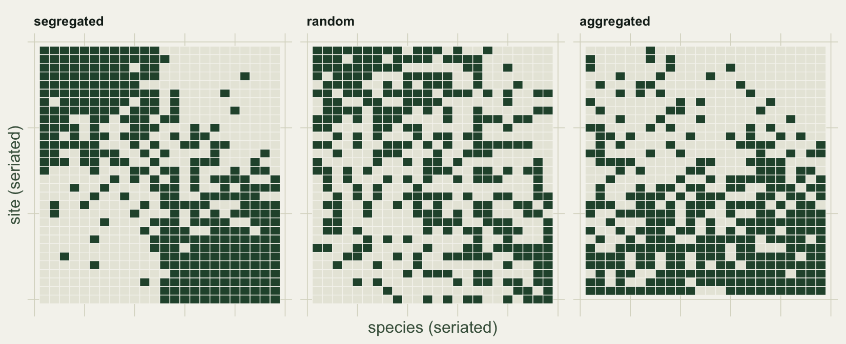
Scoring against a null model
The raw C-score cannot be read directly, because its scale depends on how common the species are and how rich the sites are. oecosimu solves this by shuffling the matrix many times under a null model, recomputing the C-score on each shuffle, and reporting where the observed value falls in that null distribution. The default tool here is the fixed-fixed null, generated by the quasiswap algorithm: it keeps both the row sums (site richness) and the column sums (species occurrence) exactly as observed, and randomizes only which cells are filled within those constraints. Gotelli (2000) compared nine such algorithms and found the fixed-fixed family the safest against false positives, which is why it is the common default.
ff <- function(M, alt){
  set.seed(42)
  oecosimu(M, nestedchecker, method = "quasiswap", nsimul = 499, alternative = alt)
}
os_seg <- ff(Seg, "greater")     # test for segregation: more checkerboards than null
os_ran <- ff(Ran, "two.sided")   # random control
os_agg <- ff(Agg, "less")        # test for aggregation: fewer checkerboards than null

ses <- function(os) as.numeric(os$oecosimu$z[1])
pval <- function(os) as.numeric(os$oecosimu$pval[1])
The standardized effect size (SES) is the observed C-score minus the null mean, divided by the null standard deviation, so it reads like a z-score: large positive means segregation, large negative means aggregation, near zero means the data sit inside the cloud of what randomness produces.
The segregated community lands far in the upper tail, with SES 82.4 and p = 0.002 (the smallest value 499 shuffles can return), so its checkerboard structure is well outside the null. The random community gives SES 0.8 and p = 0.446, sitting comfortably inside the null distribution, which is the test correctly refusing to cry wolf. The aggregated community, tested for fewer checkerboards than expected, gives SES -0.8 and p = 0.210. That is not significant. A community built so that every species shares the same sites is not flagged as aggregated.
meannull <- function(os, M) as.numeric(os$oecosimu$simulated[1, ]) / choose(ncol(M), 2)
obsmean  <- function(M) nestedchecker(M)$C.score

nulldf <- bind_rows(
  data.frame(C = meannull(os_seg, Seg), community = "segregated"),
  data.frame(C = meannull(os_agg, Agg), community = "aggregated"))
nulldf$community <- factor(nulldf$community, levels = c("segregated", "aggregated"))
obsdf <- data.frame(
  community = factor(c("segregated", "aggregated"), levels = c("segregated", "aggregated")),
  obs = c(obsmean(Seg), obsmean(Agg)),
  lab = c(sprintf("SES = %.1f\np = %.3f", ses(os_seg), pval(os_seg)),
          sprintf("SES = %.1f\np = %.3f", ses(os_agg), pval(os_agg))))

ggplot(nulldf, aes(C)) +
  geom_histogram(bins = 28, fill = line_col, color = paper, linewidth = 0.2) +
  geom_vline(data = obsdf, aes(xintercept = obs), color = red, linewidth = 0.9) +
  geom_text(data = obsdf, aes(x = obs, y = Inf, label = "observed"), color = red,
            angle = 90, hjust = 1.1, vjust = -0.4, size = 3.0) +
  geom_text(data = obsdf, aes(x = -Inf, y = Inf, label = lab), color = ink,
            hjust = -0.15, vjust = 1.5, size = 3.2, lineheight = 0.95) +
  facet_wrap(~community, scales = "free") +
  labs(x = "C-score under fixed-fixed null (mean checkerboard units per pair)",
       y = "simulations") +
  expand_limits(x = 0) + te + theme(legend.position = "none")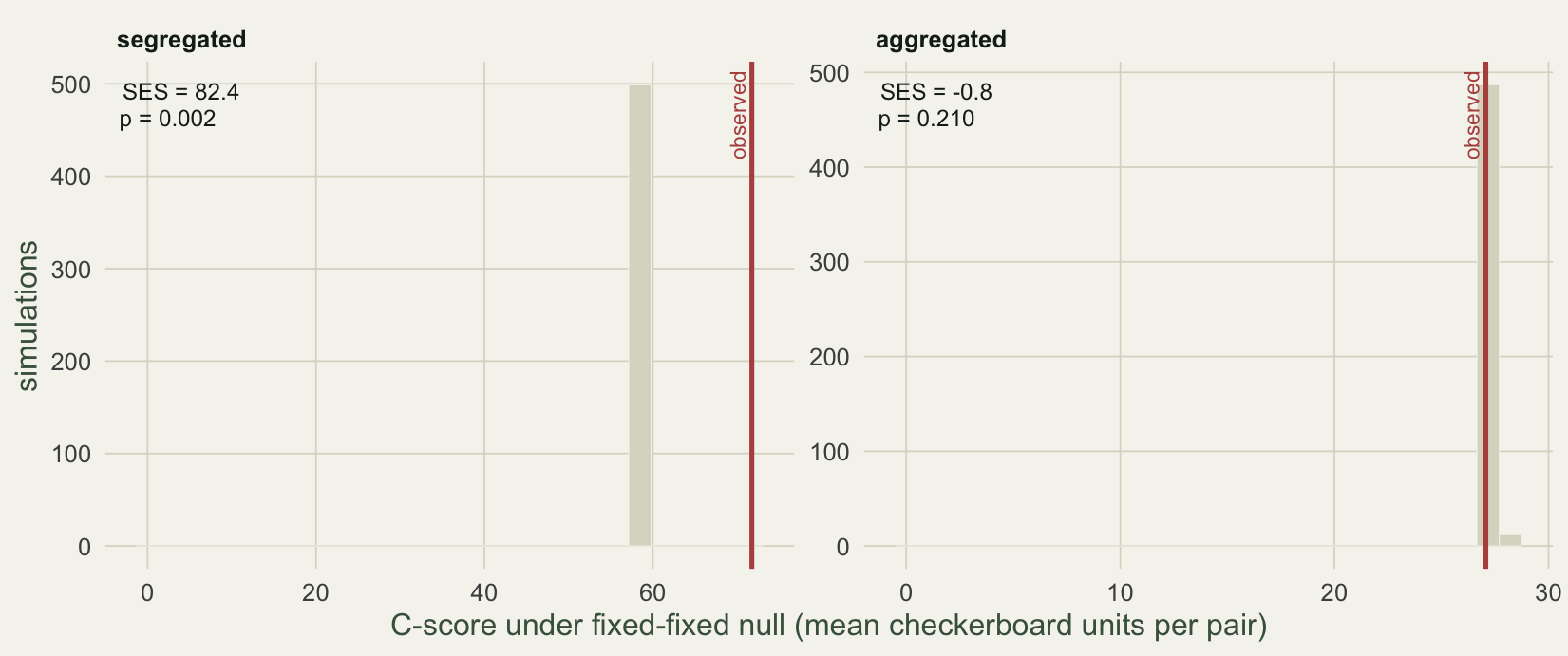
Why aggregation escapes, and what the null model decides
The non-result is not a coding accident. Aggregation, by piling species into the same good sites, makes site richness uneven: the good sites are full, the poor sites are empty. The fixed-fixed null holds those row sums fixed, so it preserves the very richness pattern that aggregation produced. Held against a null that already contains its own footprint, the observed matrix looks unremarkable. This is the conservatism Gotelli (2000) documented: the checkerboard index under a both-margins-fixed model is prone to missing real aggregation, a Type II error.
The fix and its cost become clear when you relax which margins are held. Below, the same aggregated community is tested against four null models, from the strict fixed-fixed to ones that free a margin.
methlab <- c(quasiswap = "fixed-fixed\n(quasiswap)",
             r1 = "rows fixed,\ncols proportional (r1)",
             r0 = "rows fixed,\ncols equal (r0)",
             c0 = "cols fixed,\nrows free (c0)")
zz <- c(); pp <- c()
for (m in c("quasiswap", "r1", "r0", "c0")){
  set.seed(42)
  os <- oecosimu(Agg, nestedchecker, method = m, nsimul = 499, alternative = "less")
  zz[m] <- as.numeric(os$oecosimu$z[1]); pp[m] <- as.numeric(os$oecosimu$pval[1])
}
fig3 <- data.frame(method = factor(methlab[names(zz)],
                                   levels = methlab[c("quasiswap", "r1", "r0", "c0")]),
                   SES = as.numeric(zz), p = as.numeric(pp))
fig3$sig <- ifelse(fig3$p < 0.05, "p < 0.05", "n.s.")

ggplot(fig3, aes(SES, method)) +
  geom_vline(xintercept = 0, color = faint, linewidth = 0.4) +
  geom_segment(aes(x = 0, xend = SES, yend = method), color = line_col, linewidth = 1.1) +
  geom_point(aes(color = sig), size = 4) +
  geom_text(aes(label = sprintf("p = %.3f", p)), nudge_y = 0.30, hjust = 0.5,
            color = ink, size = 3.2) +
  scale_color_manual(values = c(`p < 0.05` = forest_col, `n.s.` = faint)) +
  scale_x_continuous(limits = c(-23, 4), breaks = seq(-20, 0, 5)) +
  labs(x = "standardized effect size (SES) for aggregation", y = NULL) + te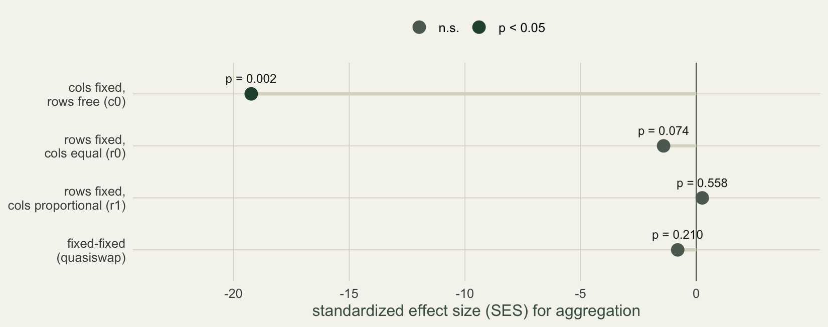
The fixed-fixed model returns SES -0.8 (p = 0.210), no signal. The r0 model, which fixes site richness but lets species occurrence vary freely, edges toward it at SES -1.4 (p = 0.074). The c0 model, which fixes species occurrence but lets site richness vary, declares strong aggregation at SES -19.2 (p = 0.002). Same matrix, opposite conclusions.
The temptation is to read c0 as the model that finally got it right. Resist it. Freeing the site-richness margin is exactly what makes a null model liberal: with richness no longer held fixed, the null compares the observed table against shuffles that have lost its real richness structure, and that mismatch alone manufactures apparent co-occurrence. Gotelli (2000) showed that algorithms which fail to preserve the richness distribution inflate false positives, so the c0 result is part real aggregation and part artifact. The lesson is not “use c0 to find aggregation.” It is that the null model is the hypothesis. The fixed-fixed model trades power for safety; relaxing it buys power at the price of false positives; and the analyst, not the software, decides which trade is acceptable for the question.
How far to read these tests
A significant C-score quantifies segregation; it does not name a cause. Diamond’s original reading was competition, but Connor & Simberloff (1979) made the durable point that the same pattern can come from dispersal limitation, shared habitat filtering, or historical accident, and that pattern alone cannot separate them. Stone & Roberts (1990) showed something sharper still: strong checkerboardedness can be produced by forces driving aggregation just as well as by avoidance, so even the sign of the departure does not map cleanly onto a mechanism. Across many real matrices, segregation is the common finding (Gotelli & McCabe 2002), but reading it as evidence of competition requires more than a low p-value.
A few practical notes. Set a seed before each oecosimu call, since the p-value comes from a finite number of shuffles and is otherwise irreproducible. With 499 simulations the smallest p-value is about 0.002, so report effect sizes alongside p-values rather than leaning on significance alone. oecosimu tracks the null distribution for the total checkerboard count and reports the per-pair C-score as a derived value; the two differ only by a constant, so the SES is identical either way. And the C-score is one of several co-occurrence indices: the number of species combinations and the variance ratio answer related but distinct questions, and the index you pick, like the null model you pick, is part of the hypothesis you are testing.
References
Diamond JM (1975). Assembly of species communities. In: Cody ML, Diamond JM (eds), Ecology and Evolution of Communities. Harvard University Press, pp 342-444.
Connor EF, Simberloff D (1979). The assembly of species communities: chance or competition? Ecology 60(6):1132-1140. doi:10.2307/1936961
Stone L, Roberts A (1990). The checkerboard score and species distributions. Oecologia 85(1):74-79. doi:10.1007/BF00317345
Gotelli NJ (2000). Null model analysis of species co-occurrence patterns. Ecology 81(9):2606-2621. doi:10.1890/0012-9658(2000)081[2606:NMAOSC]2.0.CO;2
Gotelli NJ, McCabe DJ (2002). Species co-occurrence: a meta-analysis of J. M. Diamond’s assembly rules model. Ecology 83(8):2091-2096. doi:10.1890/0012-9658(2002)083[2091:SCOAMA]2.0.CO;2
Oksanen J, Simpson G, Blanchet F, et al. (2022). vegan: Community Ecology Package. R package version 2.6-4.