Null models for phylogenetic community structure

The picante null model menu is really two questions plus a choice of species pool. Build both nulls by hand in R and see where they part company.

picante offers seven null models for ses.mpd(): taxa.labels, richness, frequency, sample.pool, phylogeny.pool, independentswap and trialswap. Choosing between them feels like a technical decision, the kind you settle by finding out which one is best.

It is not that kind of decision. The menu collapses to two questions, and picking one of them is picking your hypothesis. This post builds both from scratch and then shows the uncomfortable part: two data sets generated by opposite truths produce the same pair of answers.

Setup

Same machinery as the NRI and NTI post: a 200-species pool on a coalescent tree scaled to root depth 1, one Brownian trait.

library(ape)
library(ggplot2)

set.seed(292)
S  <- 200
tr <- rcoal(S, tip.label = sprintf("sp%03d", 1:S))
tr$edge.length <- tr$edge.length / max(node.depth.edgelength(tr))
pool  <- tr$tip.label
D     <- cophenetic(tr)[pool, pool]
trait <- rTraitCont(tr, model = "BM", sigma = 1)[pool]
trait <- (trait - mean(trait)) / sd(trait)

mpd     <- function(sp) { d <- D[sp, sp]; mean(d[lower.tri(d)]) }
mpd_row <- function(r) mpd(pool[r == 1])

The menu is shorter than it looks

Take the two nulls that sound most different. sample.pool draws a fresh set of species at random from the pool. taxa.labels leaves the community alone and shuffles the tip labels of the phylogeny instead. One randomises the ecology; the other randomises the evolution. Surely they are different tests.

set.seed(60)
comm <- sample(pool, 15)

pool_null <- replicate(4000, mpd(sample(pool, 15)))

tip_null <- replicate(4000, {
  lab <- sample(pool)
  Ds  <- D
  dimnames(Ds) <- list(lab, lab)
  d <- Ds[comm, comm]
  mean(d[lower.tri(d)])
})

c(pool_mean = mean(pool_null), tip_mean = mean(tip_null),
  pool_sd = sd(pool_null), tip_sd = sd(tip_null))

 pool_mean   tip_mean    pool_sd     tip_sd 
1.14569696 1.14398923 0.09431847 0.09092883 

ks.test(pool_null, tip_null)$p.value

[1] 0.1338343

They are the same distribution, and not approximately. Shuffling the tip labels sends your fixed set of 15 names to 15 tips chosen uniformly at random, which is what drawing 15 species at random from the pool does. For a single community whose pool is the whole tree, taxa.labels and sample.pool are one null wearing two hats.

The rest of that half of the menu differs only in which species are in the pool: everything on the tree (phylogeny.pool), or everything that occurs somewhere in your matrix (sample.pool). These are pool decisions dressed as null model decisions, and the pool gets its own sweep in the checking post.

Two of them are not even that. Run print(ses.mpd) and read the switch: the richness and sample.pool branches are the same call, both handing the matrix to randomizeMatrix(samp, null.model = "richness"). The help file describes them as different procedures, one shuffling within samples and one drawing from the pool of species observed anywhere. The source does not implement a difference. Check this yourself rather than taking my word for it, and check it before you report that a result held up across several null models.

That leaves one genuinely different family: the nulls that hold species occurrence frequency fixed.

The other question: hold occupancy fixed

independentswap shuffles the site-by-species matrix while preserving both margins. Row sums stay put, so every site keeps its richness. Column sums stay put, so every species keeps the number of sites it occupies. The move is the checkerboard swap: find a two-by-two submatrix reading 1,0 / 0,1 and flip it.

swap_n <- function(M, n, B = 300) {
  R <- nrow(M); Cc <- ncol(M); done <- 0
  while (done < n) {
    i1 <- sample(R, B, TRUE); i2 <- sample(R, B, TRUE)
    j1 <- sample(Cc, B, TRUE); j2 <- sample(Cc, B, TRUE)
    a  <- M[cbind(i1, j1)]; b  <- M[cbind(i1, j2)]
    c2 <- M[cbind(i2, j1)]; d  <- M[cbind(i2, j2)]
    hit <- which(i1 != i2 & j1 != j2 &
                 ((a == 1 & b == 0 & c2 == 0 & d == 1) |
                  (a == 0 & b == 1 & c2 == 1 & d == 0)))
    for (h in hit) {
      if (done >= n) break
      if (M[i1[h], j1[h]] == a[h] && M[i1[h], j2[h]] == b[h] &&
          M[i2[h], j1[h]] == c2[h] && M[i2[h], j2[h]] == d[h]) {
        M[i1[h], j1[h]] <- 1 - a[h];  M[i1[h], j2[h]] <- 1 - b[h]
        M[i2[h], j1[h]] <- 1 - c2[h]; M[i2[h], j2[h]] <- 1 - d[h]
        done <- done + 1
      }
    }
  }
  M
}

The batched candidate search is only a speed trick: the fill here is under eight per cent, so a randomly picked two-by-two is a valid checkerboard about one per cent of the time, and drawing 300 candidates at once beats a rejection loop. The same swap machinery drives the C-score tests in the co-occurrence null model post; what changes here is the statistic laid on top of it.

The two nulls, wrapped up:

ses_pool <- function(M, R = 199) {
  sapply(seq_len(nrow(M)), function(i) {
    k <- sum(M[i, ]); o <- mpd_row(M[i, ])
    nul <- replicate(R, mpd(sample(pool, k)))
    -(o - mean(nul)) / sd(nul)
  })
}

ses_swap <- function(M, R = 199, iter = 200) {
  obs <- apply(M, 1, mpd_row)
  nul <- matrix(NA_real_, R, nrow(M))
  X   <- swap_n(M, 5000)                       # burn-in away from the observed matrix
  for (r in 1:R) { X <- swap_n(X, iter); nul[r, ] <- apply(X, 1, mpd_row) }
  -(obs - colMeans(nul)) / apply(nul, 2, sd)
}

Both return NRI per site, so positive still means clustered.

Three data sets

Forty sites, fifteen species each, drawn from the same 200-species pool three different ways.

nt   <- node.depth(tr)[-(1:S)]                # species descending from each internal node
node <- (which(nt >= 40 & nt <= 45) + S)[1]   # first clade holding 40 to 45 species
wide <- extract.clade(tr, node)$tip.label

draw <- function(seed, prob_i) {
  set.seed(seed)
  M <- matrix(0L, 40, S, dimnames = list(NULL, pool))
  for (i in 1:40) M[i, sample(S, 15, prob = prob_i(i))] <- 1L
  M
}

# A: no local process at all. Every site is the same weighted draw, and one
#    clade is six times as likely to turn up as anything else.
pw <- ifelse(pool %in% wide, 6, 1)
M1 <- draw(41, function(i) pw)

# B: real habitat filtering, sites differ in what they select for.
set.seed(42); optB <- rnorm(40)
M2 <- draw(421, function(i) exp(-(trait - optB[i])^2 / (2 * 0.5^2)))

# C: real habitat filtering, but every site is nearly the same habitat.
set.seed(43); optC <- rnorm(40, 1.2, 0.25)
M3 <- draw(431, function(i) exp(-(trait - optC[i])^2 / (2 * 0.5^2)))

Matrix A has no assembly rule whatsoever. Each site is an independent weighted draw from one fixed distribution, and 42 of the 200 species are widespread because they belong to one clade. Nothing about a site decides who arrives. Matrix B is genuine environmental filtering with sites spread over the trait axis. Matrix C is genuine environmental filtering too, but all forty sites are nearly the same habitat, so the same species win everywhere.

Naming the widespread clade rather than letting a random trait supply one is deliberate. An earlier draft drew occupancy as a Brownian trait, which conserves occupancy in expectation but not reliably: across twelve independent draws of that trait on this tree, eleven produced communities pulled towards relatives and one produced the opposite. A data set whose sign depends on which draw you got is not a demonstration. Weighting a named clade makes the claim checkable before any null runs:

exp_mpd <- function(w) { W <- outer(w, w); diag(W) <- 0; sum(W * D) / sum(W) }
c(uniform = exp_mpd(rep(1, S)), weighted_A = exp_mpd(pw))

   uniform weighted_A 
 1.1449617  0.9292778 

The weights pull the expected pairwise distance below the uniform value, so matrix A really will look clustered to a null that assumes uniform draws. That is the trap being built.

set.seed(51); p1 <- ses_pool(M1); set.seed(52); s1 <- ses_swap(M1)
set.seed(53); p2 <- ses_pool(M2); set.seed(54); s2 <- ses_swap(M2)
set.seed(55); p3 <- ses_pool(M3); set.seed(56); s3 <- ses_swap(M3)

pct <- function(x) round(100 * mean(abs(x) > 1.96))
data.frame(
  matrix     = c("A no local process", "B filtering, mixed sites", "C filtering, one habitat"),
  pool_NRI   = round(c(mean(p1), mean(p2), mean(p3)), 2),
  pool_pct   = c(pct(p1), pct(p2), pct(p3)),
  swap_NRI   = round(c(mean(s1), mean(s2), mean(s3)), 2),
  swap_pct   = c(pct(s1), pct(s2), pct(s3))
)

                    matrix pool_NRI pool_pct swap_NRI swap_pct
1       A no local process     1.79       55    -0.05        0
2 B filtering, mixed sites     2.96       57     3.22       62
3 C filtering, one habitat     3.64       82     0.09        2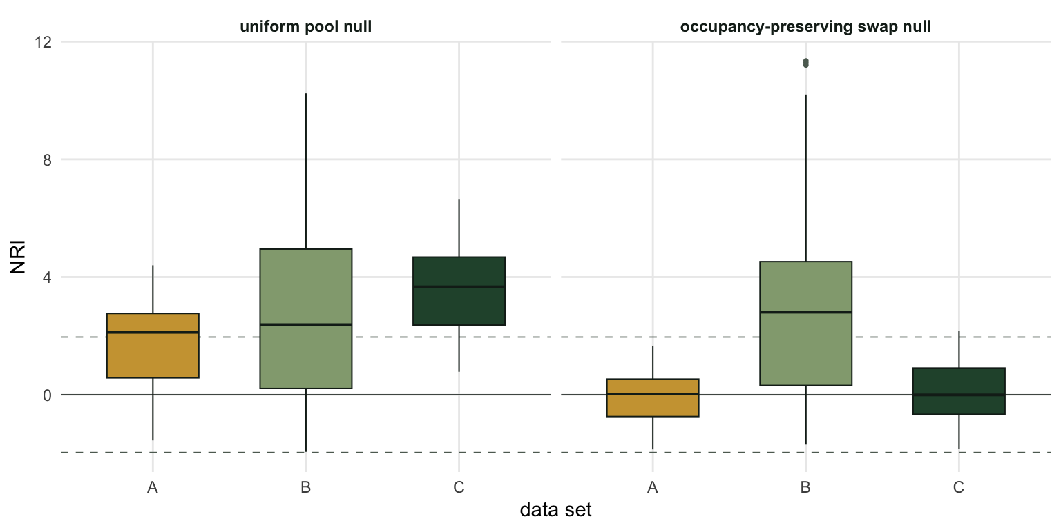

Figure 1: NRI across 40 sites under the two nulls, for three data sets. Rows A and C give the same pair of answers from opposite truths: A has no local assembly process, C has a strong one.

Reading the table

Start with row B, the reassuring one. Filtering is real, sites differ, and both nulls find it: pool NRI +2.96, swap NRI +3.22. Holding occupancy fixed cost nothing here, because the occupancy pattern this process produced carries almost no phylogenetic information. The most widespread species occurs at 7 of the 40 sites; there is nothing for the swap null to absorb.

Row A is the classic warning. Nothing assembled these communities. Every site drew from the same distribution, independently, with no interaction, no environment and no history. The pool null reports NRI +1.79 and flags 55 per cent of sites as significantly clustered. It is not malfunctioning: the communities really are not uniform draws from the pool, because common species are common. But “not a uniform draw from the pool” is not “assembled by a local process”, and the arrow from one to the other is where the inference breaks. The swap null, which already knows that common species are common, reports NRI -0.05.

Now row C, and this is the part worth sitting with. Filtering is real and strong. Every site selects on a conserved trait. The pool null sees it: NRI +3.64, 82 per cent of sites flagged, the strongest signal in the table. The swap null reports +0.09 and flags 2 per cent.

The swap null has not made an error. Because every site is the same habitat, the filtering is the occupancy pattern: the species that suit the habitat are widespread (the commonest occurs at 17 of the 40 sites, against 7 in row B), and they are relatives. Conditioning on occupancy conditions on the process. The swap null answers “given how widespread each species is, do these sites contain more related species than a reshuffle would give?”, and the answer is honestly no.

Put rows A and C side by side. Same pool null verdict (strong clustering), same swap null verdict (nothing), opposite truths. The choice of null did not resolve the question. It named which question was asked.

The honest limit

There is no default null model, and the search for the one that “controls for” the nuisance is a search for something that does not exist. Every null is a hypothesis about what would have happened otherwise, and a site-by-species matrix plus a tree does not contain enough information to choose between the hypotheses in rows A and C. It never will, because the two processes leave the same footprint.

What does help is nothing you can compute from the matrix: knowing whether the sites differ environmentally, whether the widespread species are widespread for reasons connected to the sites you sampled, and what the pool means. Report both nulls, say what each one holds fixed, and let the difference between them be a finding rather than something you resolve by picking a winner.

Where to go next

The nulls so far all answer a within-community question. Swap the question to a between-community one and the same tree and distance matrix produce phylogenetic beta diversity, where the surprise is that two communities can share no species at all and still be nearly identical.

Related tutorials

• Phylogenetic community structure: NRI and NTI in R
• Phylogenetic beta diversity: UniFrac and PhyloSor
• Checking a community phylogenetics analysis
• Species co-occurrence null models

References

• Webb, Ackerly, McPeek, Donoghue 2002 Annual Review of Ecology and Systematics 33:475-505 (10.1146/annurev.ecolsys.33.010802.150448)
• Hardy 2008 Journal of Ecology 96(5):914-926 (10.1111/j.1365-2745.2008.01421.x)
• Kembel 2009 Ecology Letters 12(9):949-960 (10.1111/j.1461-0248.2009.01354.x)
• Miller, Farine, Trisos 2017 Ecography 40(4):461-477 (10.1111/ecog.02070)