library(ape)
library(ggplot2)
te_canvas <- theme(plot.background  = element_rect(fill = "#f5f4ee", colour = NA),
                   panel.background = element_rect(fill = "#f5f4ee", colour = NA))

set.seed(292)
S <- 200
pool_tree <- rcoal(S, tip.label = sprintf("sp%03d", 1:S))
pool_tree$edge.length <- pool_tree$edge.length / max(node.depth.edgelength(pool_tree))
pool <- pool_tree$tip.label

D <- cophenetic(pool_tree)[pool, pool]
trait <- rTraitCont(pool_tree, model = "BM", sigma = 1)[pool]
trait <- (trait - mean(trait)) / sd(trait)Phylogenetic community structure: NRI and NTI in R
R
community phylogenetics
biodiversity
ggplot2
ecology tutorial
Raw MPD and MNTD are confounded with species richness in a plot. Build standardised effect sizes, NRI and NTI, by hand in R and learn to read their signs.
Corrected 8 October 2026: the post explained the wide spread of the filtered NRI by trait optima landing in crowded or empty parts of the pool, which the runs do not bear out, and said that the spacing rule rejects candidates close to a resident; it now puts the spread down to where each optimum falls and says that the rule down-weights close candidates.
Corrected 1 October 2026: the post called the index calibrated on the strength of its mean and spread, pointed to the checking post for a case it does not contain, and said that limiting similarity showing up mainly in NTI follows from the metrics alone; it now notes that the skewed MNTD null puts the dashed cut-offs off their nominal rates and that the spacing rule here acts directly on distances in the tree.
You have a species list for a plot and a phylogeny for the regional flora. Are the species in that plot closer relatives than you would expect, and if so, does that say anything about how the community was assembled?
The metric part of this question is easy. The interpretive part is where the whole field lives, and it starts with a fact that is easy to miss: the raw number you compute from a plot is not a property of the plot. For MNTD it is mostly a property of how many species the plot has, and even for MPD how unusual a given value is depends on the species count.
This post builds the standard fix from scratch: the standardised effect size, and its two sign-flipped aliases, the Net Relatedness Index (NRI) and the Nearest Taxon Index (NTI). Everything is base R plus ape for the tree.
Setup
A regional pool of 200 species on a coalescent tree, scaled so the root sits at depth 1 (the largest possible distance between two tips is therefore 2). One trait evolves on the tree under Brownian motion, so close relatives resemble each other: that is the assumption the whole method rests on, and it is worth naming out loud.
cophenetic() gives the patristic distance matrix: the summed branch length on the path between each pair of tips. Everything below reads from that matrix and nothing else.
Two distances, two depths
Two summaries dominate the literature, and they are two lines each.
mpd <- function(sp) { d <- D[sp, sp]; mean(d[lower.tri(d)]) }

mntd <- function(sp) {
  d <- D[sp, sp]
  diag(d) <- NA
  mean(apply(d, 1, min, na.rm = TRUE))
}
Mean pairwise distance (MPD) averages over every pair in the community. Mean nearest taxon distance (MNTD) averages, over each species, the distance to its single closest relative in the community.
They are not two flavours of the same thing. MPD is dominated by the deep splits: swap one species for a member of a distant clade and every pair involving it changes. MNTD only looks at each species’ nearest neighbour, so it is a measurement of the terminal structure. A community can be built from two distant clades (high MPD) with tight species clusters inside each (low MNTD). Keep that picture; it explains most of the confusing results later.
The raw number depends on richness
Here is the experiment nobody runs before reporting an MNTD. Draw communities at random from the pool at five richness levels, with no assembly rule whatsoever, and look at what the raw metrics do.
neutral <- function(k) sample(pool, k)

set.seed(1)
kg <- rep(c(4, 8, 15, 25, 40), each = 200)
raw <- t(sapply(kg, function(k) { s <- neutral(k); c(mpd(s), mntd(s)) }))
tab <- data.frame(
  k      = sort(unique(kg)),
  mpd_m  = tapply(raw[, 1], kg, mean), mpd_s  = tapply(raw[, 1], kg, sd),
  mntd_m = tapply(raw[, 2], kg, mean), mntd_s = tapply(raw[, 2], kg, sd)
)
round(tab, 3)
k mpd_m mpd_s mntd_m mntd_s
4 4 1.129 0.287 0.634 0.243
8 8 1.129 0.183 0.342 0.135
15 15 1.144 0.091 0.204 0.074
25 25 1.142 0.064 0.129 0.044
40 40 1.150 0.046 0.084 0.026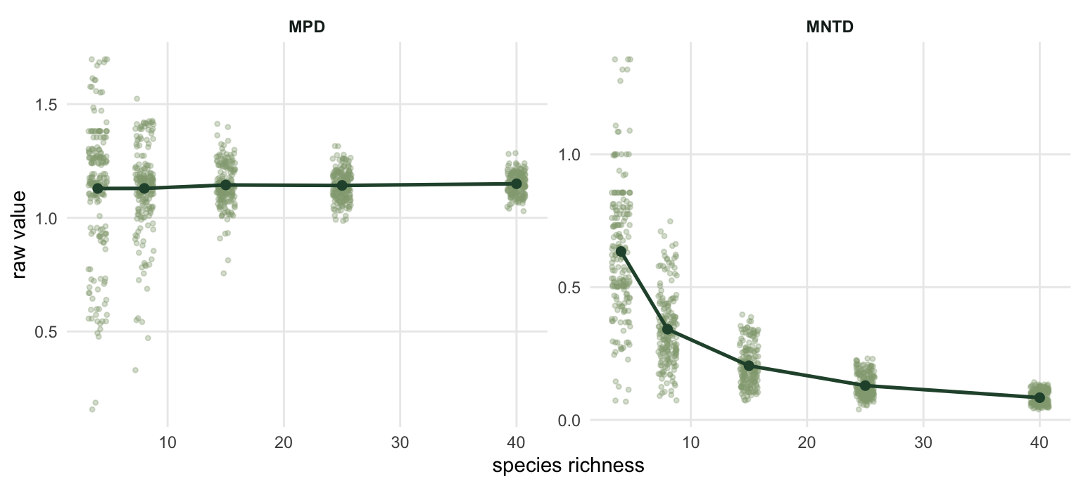
The MNTD mean falls by a factor of 7.57 between richness 4 and richness 40. Nothing ecological happened. Add species to a fixed pool and each species’ nearest relative simply gets nearer, because there are more candidates. Any comparison of raw MNTD between a species-poor plot and a species-rich plot is a comparison of richness wearing a phylogenetic costume.
MPD looks safer at first: the mean barely moves (1.13 to 1.15). But look at the second column. The standard deviation shrinks by a factor of 6.21 over the same range. A four-species plot sitting 0.2 below the pool mean is unremarkable; a forty-species plot sitting 0.2 below it is extraordinary. The raw deviation means different things at different richness, which is the same problem in a quieter voice.
Standardising against a null
The fix is the obvious one. Ask what the metric would look like if this community, with exactly this richness, had been drawn at random from the pool, and express the observation in units of that distribution.
ses <- function(sp, R = 999) {
  k   <- length(sp)
  obs <- c(mpd(sp), mntd(sp))
  nul <- replicate(R, { s <- sample(pool, k); c(mpd(s), mntd(s)) })
  z   <- (obs - rowMeans(nul)) / apply(nul, 1, sd)
  p   <- (rowSums(nul <= obs) + 1) / (R + 1)
  list(obs = obs, null = nul, z = z, p = p, nri = -z[1], nti = -z[2])
}
Three conventions are buried in those few lines, and each one has cost somebody a paragraph in review.
The sign is flipped. NRI is defined as minus the standardised MPD, and NTI as minus the standardised MNTD. So positive NRI means clustering: the community is more closely related than chance, which is a low MPD. If you report ses.mpd from picante and then discuss it as if it were NRI, every sign in your discussion is backwards. This is the single most common slip in the method.
The p-value is a rank, not a z-test. The p line counts how many null draws fall at or below the observation. That works whatever shape the null distribution has, which matters more than it sounds: the MNTD null in the figure below is skewed to the right, and for a skewed null a z-score cut-off and the rank p-value can disagree.
The null is a decision, not a default. Here the null draws species uniformly from the pool. That is one hypothesis out of several, and it is the subject of the next post.
Three assembly rules, three signatures
Now build communities under three rules and see what the index reports. Habitat filtering picks species whose trait is near a local optimum. Limiting similarity picks species that are far from whatever has already been picked. The neutral rule picks at random.
filtered <- function(k, opt, w = 0.3) {
  sample(pool, k, prob = exp(-(trait - opt)^2 / (2 * w^2)))
}

spaced <- function(k) {
  sel <- sample(pool, 1)
  while (length(sel) < k) {
    cand <- setdiff(pool, sel)
    sel  <- c(sel, sample(cand, 1, prob = apply(D[cand, sel, drop = FALSE], 1, min)^8))
  }
  sel
}

set.seed(10); cf <- filtered(15, 1.2)
set.seed(11); cn <- neutral(15)
set.seed(12); co <- spaced(15)

set.seed(20); sf <- ses(cf)
set.seed(21); sn <- ses(cn)
set.seed(22); so <- ses(co)

data.frame(
  rule = c("filtered", "neutral", "spaced"),
  MPD  = round(c(sf$obs[1], sn$obs[1], so$obs[1]), 3),
  NRI  = round(c(sf$nri, sn$nri, so$nri), 2),
  MNTD = round(c(sf$obs[2], sn$obs[2], so$obs[2]), 3),
  NTI  = round(c(sf$nti, sn$nti, so$nti), 2)
)
rule MPD NRI MNTD NTI
1 filtered 0.724 4.67 0.029 2.29
2 neutral 1.123 0.20 0.140 0.85
3 spaced 1.294 -1.62 0.433 -3.25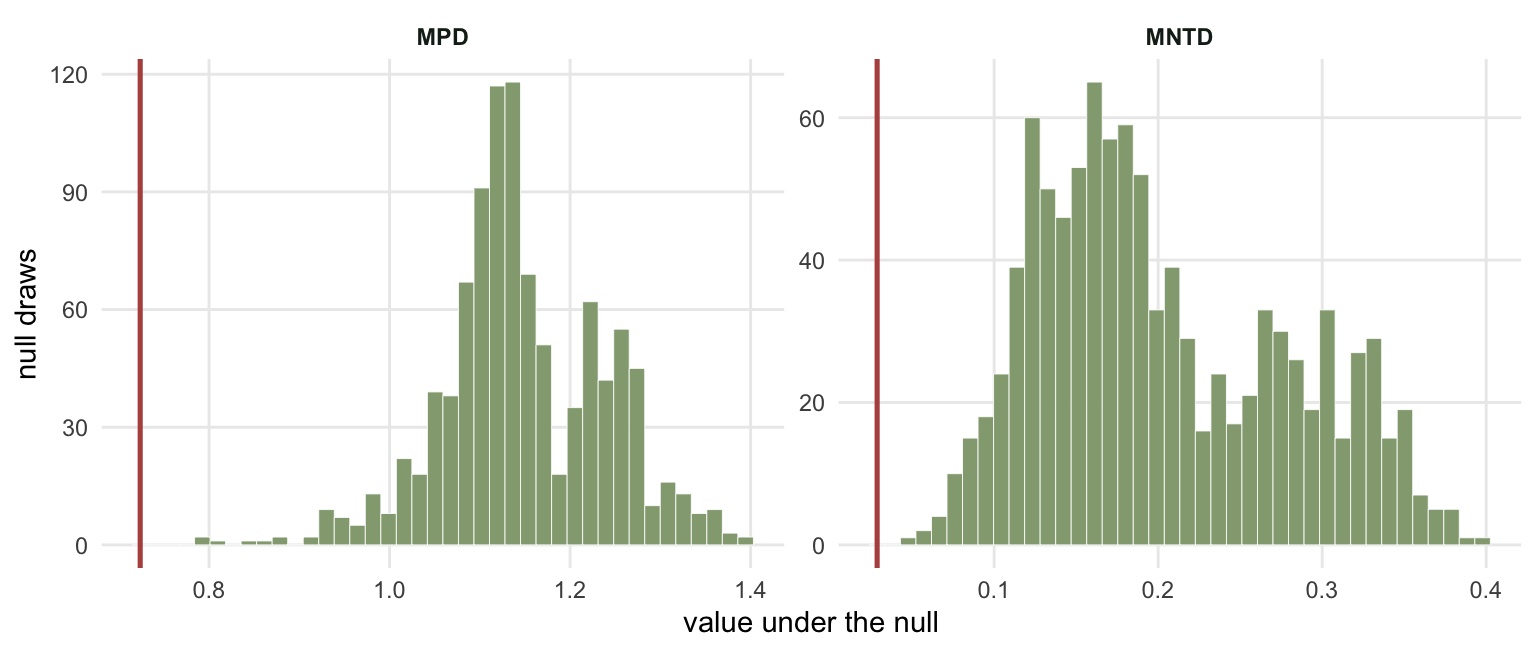
The filtered community, which really was assembled by filtering, lands at NRI +4.67 with a rank p of 0.001. The neutral community lands at NRI +0.20, p 0.424, against a truth of no structure at all. The spaced community lands at NTI -3.25: overdispersed at the tips.
Repeat over 100 communities per rule to see how reliable that is.
rep_ses <- function(gen, n = 100, R = 199) {
  t(replicate(n, {
    sp  <- gen(15)
    obs <- c(mpd(sp), mntd(sp))
    nul <- replicate(R, { s <- sample(pool, 15); c(mpd(s), mntd(s)) })
    -(obs - rowMeans(nul)) / apply(nul, 1, sd)
  }))
}

set.seed(30); A <- rep_ses(function(k) filtered(k, rnorm(1)))
set.seed(31); B <- rep_ses(neutral)
set.seed(32); C <- rep_ses(spaced)

data.frame(
  rule    = c("filtered", "neutral", "spaced"),
  NRI     = round(c(mean(A[, 1]), mean(B[, 1]), mean(C[, 1])), 2),
  NRI_sd  = round(c(sd(A[, 1]), sd(B[, 1]), sd(C[, 1])), 2),
  NTI     = round(c(mean(A[, 2]), mean(B[, 2]), mean(C[, 2])), 2),
  NTI_sd  = round(c(sd(A[, 2]), sd(B[, 2]), sd(C[, 2])), 2)
)
rule NRI NRI_sd NTI NTI_sd
1 filtered 3.39 3.76 1.33 0.90
2 neutral 0.06 1.09 0.17 1.04
3 spaced -1.57 0.13 -3.09 0.18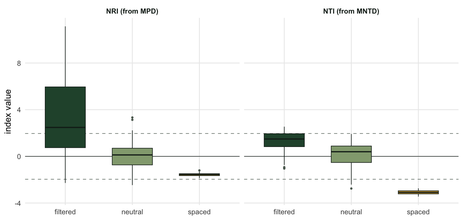
The neutral row is the one to read first. Its NRI averages +0.06 with a spread of 1.09, and its NTI averages +0.17 with a spread of 1.04. Centred on zero, spread of about one: that is what a standardised effect size is supposed to do when the data really were generated by the null. Centre and spread are not the whole story, though: the MNTD null is skewed to the right (the figure above), so under the null NTI almost never reaches the upper dashed line and passes the lower one a little more often than a normal curve would. The rank p-value, which assumes no shape, is the one to test with.
Why NRI and NTI disagree
Now the asymmetry. Habitat filtering shows up mainly in NRI (+3.39, against +1.33 for NTI). Limiting similarity shows up mainly in NTI (-3.09, against -1.57 for NRI).
Part of that is built into these simulations. A conserved trait varies most between distant clades, so filtering on it selects whole clades and collapses the deep structure, which is exactly what MPD sees. The spacing rule here down-weights each candidate the closer it sits in the tree to its nearest resident, so it acts on nearest neighbours, which is exactly what MNTD sees; a rule that spaced species on the trait instead would reach the tree only through the trait, and need not leave the same mark on NTI. The two indices are not redundant, and a paper reporting only one of them has answered only one of the two questions.
Two more things in that table deserve a mention. The filtered NRI has a spread of 3.76, far wider than the other rules, because each filtered community has its own randomly placed trait optimum, and how clustered the community comes out depends heavily on where that optimum falls. And the spaced rule produces a very tight distribution, because the draw that builds it is weighted so heavily towards species far from every resident that the index barely moves, even though the species picked differ from one community to the next. Effect size and its variability are separate facts about a process.
The honest limit
The number that came out of ses() is not “how clustered this community is”. It is “how clustered this community is relative to a uniform draw from these 200 species”. Change the 200 and the answer changes, and there is no data-internal test that tells you which 200 is right. Everything downstream inherits this. The tree inherits it too: swap the tree and the distances move.
The method is worth using anyway, because the alternative is reading raw MNTDs across plots of unequal richness, which measures nothing at all. But the standardised number is a statement about a comparison you chose, not a discovery about nature. The checking post makes that concrete by moving the pool and watching the conclusion move with it.
Where to go next
The obvious next question is the one this post kept deferring: which null? Drawing uniformly from the pool is not the only option, and the alternatives ask genuinely different questions rather than being better or worse approximations of one question. That comes next. After that, the same tree and the same distance matrix answer a between-community question instead of a within-community one.
References
- Webb 2000 American Naturalist 156(2):145-155 (10.1086/303378)
- Webb, Ackerly, McPeek, Donoghue 2002 Annual Review of Ecology and Systematics 33:475-505 (10.1146/annurev.ecolsys.33.010802.150448)
- Webb, Ackerly, Kembel 2008 Bioinformatics 24:2098-2100 (10.1093/bioinformatics/btn358)
- Kembel, Cowan, Helmus, Cornwell, Morlon, Ackerly, Blomberg, Webb 2010 Bioinformatics 26(11):1463-1464 (10.1093/bioinformatics/btq166)