Phylogenetic beta diversity: UniFrac and PhyloSor

Two communities can share no species and still be nearly identical. Build UniFrac and PhyloSor by hand in R, and find they are one metric wearing two names.

Two plots share no species at all. Sorensen dissimilarity is 1, and it would still be 1 if one plot held ten oaks and the other held ten different oaks, or if one held ten oaks and the other held ten mosses. The metric cannot tell those situations apart because it never learned that species are related to each other.

Phylogenetic beta diversity fixes that by counting branch length instead of species. This post builds the two standard versions from scratch, and then finds that they were never two versions.

Setup

The same 200-species pool used in the NRI and NTI post.

library(ape)
library(ggplot2)

set.seed(292)
S  <- 200
tr <- rcoal(S, tip.label = sprintf("sp%03d", 1:S))
tr$edge.length <- tr$edge.length / max(node.depth.edgelength(tr))
pool <- tr$tip.label

sorensen <- function(a, b) 2 * length(intersect(a, b)) / (length(a) + length(b))

Branch length accounting

Every metric here needs one thing: for each branch of the tree, which communities have a species descending from it. Walk the edge matrix backwards, since ape stores edges with parents before children, and accumulate the descendant tips.

desc_tips <- function(tr) {
  out <- vector("list", max(tr$edge))
  for (i in seq_len(Ntip(tr))) out[[i]] <- i
  for (e in rev(seq_len(nrow(tr$edge)))) {
    p <- tr$edge[e, 1]; ch <- tr$edge[e, 2]
    out[[p]] <- c(out[[p]], out[[ch]])
  }
  out
}
DT <- desc_tips(tr)

branch_flags <- function(sp) {
  idx <- match(sp, tr$tip.label)
  vapply(tr$edge[, 2], function(ch) any(DT[[ch]] %in% idx), logical(1))
}

branch_flags() returns one TRUE or FALSE per branch: does this community reach down through that branch. Everything else is bookkeeping on three numbers. Write s for the branch length shared by both communities, and PD for the total branch length a community spans, root included.

pbd <- function(a, b) {
  A <- branch_flags(a); B <- branch_flags(b); L <- tr$edge.length
  s  <- sum(L[A & B])
  pa <- sum(L[A]); pb <- sum(L[B])
  c(unifrac  = (pa + pb - 2 * s) / (pa + pb - s),
    phylosor = 2 * s / (pa + pb))
}

Unweighted UniFrac is the share of branch length that only one of the two communities reaches. PhyloSor is the Sorensen formula with branch length in place of species counts. Both ignore abundance; both need the root, a point returned to below.

Zero shared species, two different answers

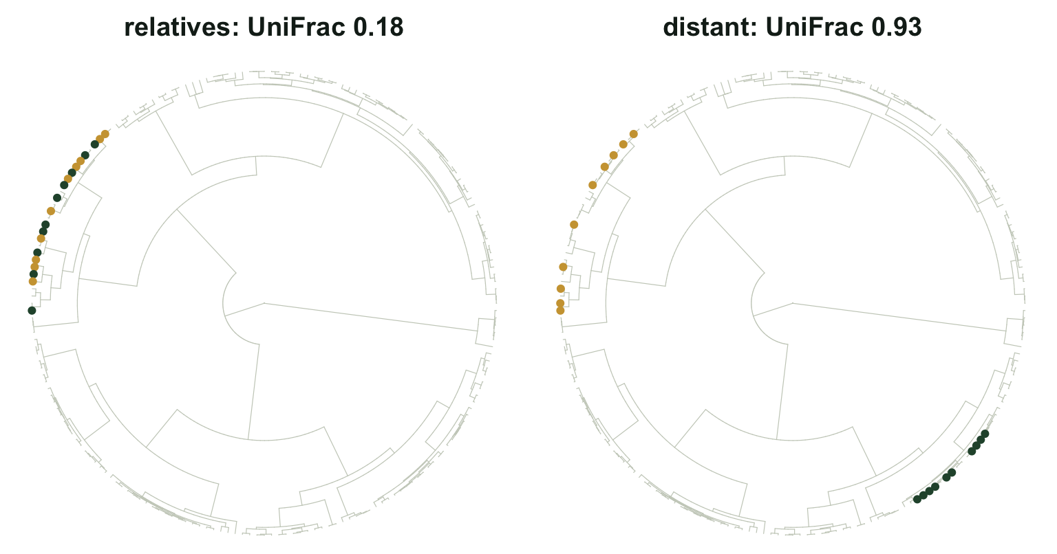
Build two pairs of communities, each pair sharing not a single species. The first pair lives inside one clade; the second pair sits on opposite sides of the tree.

nt    <- node.depth(tr)[-(1:S)]
cands <- which(nt >= 20 & nt <= 30) + S
cl1   <- extract.clade(tr, cands[1])$tip.label
cl2   <- extract.clade(tr, cands[length(cands)])$tip.label

set.seed(7)
near_a <- sample(cl1, 10); near_b <- sample(setdiff(cl1, near_a), 10)
far_a  <- sample(cl1, 10); far_b  <- sample(cl2, 10)

rbind(relatives = c(sorensen = sorensen(near_a, near_b), pbd(near_a, near_b)),
      distant   = c(sorensen = sorensen(far_a,  far_b),  pbd(far_a,  far_b)))

          sorensen   unifrac  phylosor
relatives        0 0.1750607 0.9040732
distant          0 0.9253535 0.1389228

Sorensen reports zero similarity for both pairs, which is correct and useless. UniFrac separates them: 0.175 for the pair of relatives against 0.925 for the distant pair. The first pair overlaps on almost all of its branch length despite overlapping on none of its species.

Figure 1: The same Sorensen value, two situations. Left: both communities drawn from one clade, sharing no species. Right: communities drawn from clades on opposite sides of the tree, also sharing no species.

The two metrics are one metric

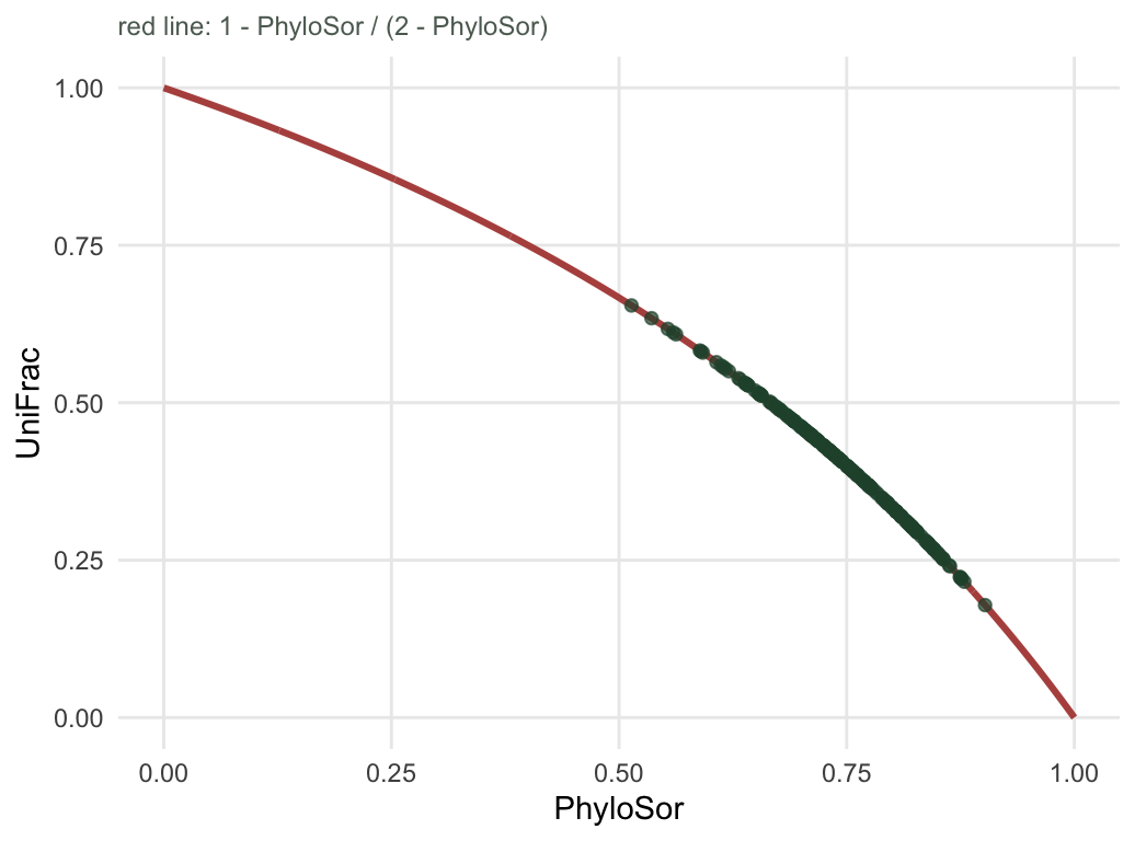
UniFrac and PhyloSor look like alternatives, and papers report one or the other as though something turned on the choice. Put the branch bookkeeping in the same notation as the species bookkeeping and the alternative disappears. With s for shared branch length and u for the branch length unique to one side or the other, PhyloSor is 2s/(2s+u), the Sorensen form, and UniFrac is u/(s+u), which is one minus the Jaccard form. Sorensen and Jaccard have a fixed algebraic relationship, so these do too.

set.seed(8)
z <- t(replicate(200, {
  a <- sample(pool, sample(5:30, 1))
  b <- sample(pool, sample(5:30, 1))
  pbd(a, b)
}))
all.equal(z[, "unifrac"], 1 - z[, "phylosor"] / (2 - z[, "phylosor"]))

[1] TRUE

cor(z[, "unifrac"], z[, "phylosor"], method = "spearman")

[1] -1

Not correlated, not usually similar: equal, to machine precision, on every pair. Each metric is a deterministic function of the other. A study that reports UniFrac and a study that reports PhyloSor have reported the same number twice, and any ordering of community pairs is identical under both. The rank correlation of exactly negative one is the whole story.

Figure 2: Every random pair of communities falls exactly on the curve relating the two metrics. There is no scatter to explain.

This is the same finding as the null model post, where four of picante’s eight null models turned out to be one null model plus a choice of species pool. The menus in community phylogenetics are shorter than they advertise.

The same richness problem as before

The NRI post showed raw MNTD falling steeply with richness, which is why nobody reports raw MNTD. UniFrac has the identical problem, and it is reported raw constantly.

set.seed(9)
ks <- c(5, 10, 20, 40, 80)
rd <- do.call(rbind, lapply(ks, function(k) {
  data.frame(k = k, uf = replicate(60, pbd(sample(pool, k), sample(pool, k))[["unifrac"]]))
}))
ggplot(rd, aes(factor(k), uf)) +
  geom_jitter(width = 0.15, colour = "#93a87f", size = 1.1, alpha = 0.6) +
  stat_summary(aes(group = 1), fun = mean, geom = "line", colour = "#275139", linewidth = 0.9) +
  stat_summary(fun = mean, geom = "point", colour = "#275139", size = 2.2) +
  labs(x = "species per community", y = "UniFrac") +
  theme_minimal(base_size = 11) +
  theme(panel.grid.minor = element_blank())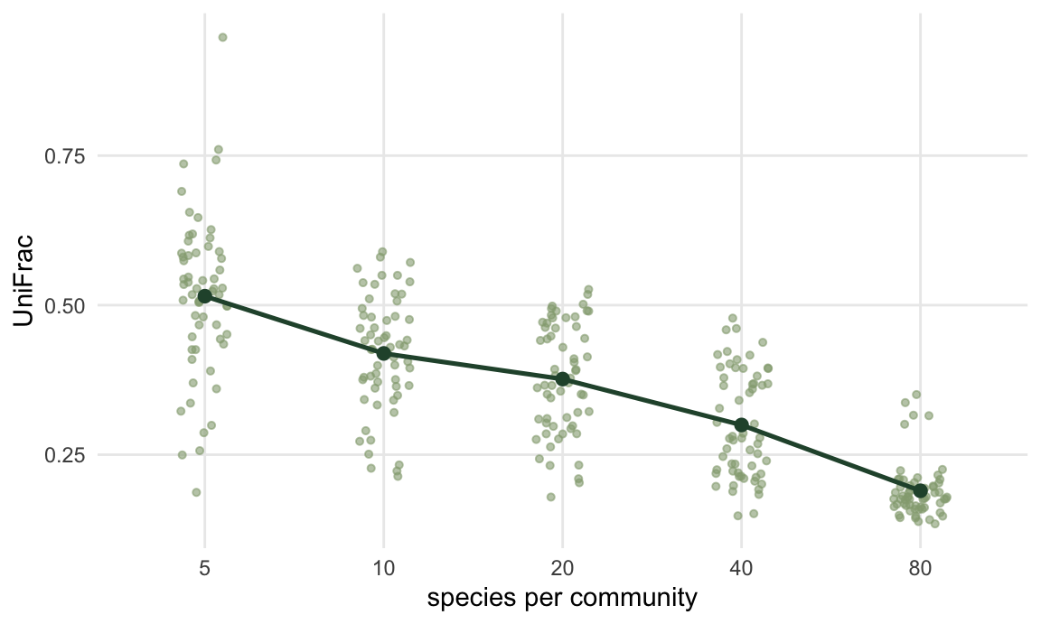

Figure 3: UniFrac between two communities drawn at random from the same pool, against the richness of each. Nothing differs between these communities except how many species they contain.

aggregate(uf ~ k, rd, function(x) round(c(mean = mean(x), sd = sd(x)), 3))

   k uf.mean uf.sd
1  5   0.515 0.133
2 10   0.419 0.095
3 20   0.376 0.092
4 40   0.300 0.089
5 80   0.190 0.046

Two communities of five random species look 2.7 times more dissimilar than two communities of eighty random species, and both pairs were generated by exactly the same process. Richer communities cover more of the tree, so they overlap on more branch length, so UniFrac falls. If your sites differ in richness (they do), a UniFrac matrix has a richness gradient baked into it, and any ordination of that matrix will find the gradient and offer it to you as ecology.

The fix is the one from the NRI post: compare each observed value against a null distribution built at the observed richness, and report the standardised effect size rather than the raw number. It is more code and a slower analysis, and it is not optional.

The honest limit

Both metrics need a root, and the root is a modelling choice rather than an observation. Branch length above the deepest split in your sample gets counted as shared by everything, which drags all values towards similarity when your pool is deep and shallow when it is not. Unrooted UniFrac exists, answers a slightly different question, and is not interchangeable with what is built here.

The bigger limit is what the metrics are silent about. A low UniFrac says two communities occupy the same part of the tree. It does not say why, and the two explanations that matter, shared environment and shared history, produce the same branch length overlap. That is the same wall the null model post ran into, and no beta diversity metric climbs it.

Where to go next

Three posts in, the tools work and the numbers come out. What is missing is the set of checks that decide whether any of it means anything: pool sensitivity, tree error, and the question of whether the effect survives the assumptions.

Related tutorials

• Phylogenetic community structure: NRI and NTI in R
• Null models for phylogenetic community structure
• Checking a community phylogenetics analysis
• Phylogenetic diversity with picante

References

• Lozupone, Knight 2005 Applied and Environmental Microbiology 71(12):8228-8235 (10.1128/AEM.71.12.8228-8235.2005)
• Lozupone, Hamady, Kelley, Knight 2007 Applied and Environmental Microbiology 73(5):1576-1585 (10.1128/AEM.01996-06)
• Bryant, Lamanna, Morlon, Kerkhoff, Enquist, Green 2008 Proceedings of the National Academy of Sciences 105(Supplement 1):11505-11511 (10.1073/pnas.0801920105)
• Graham, Fine 2008 Ecology Letters 11(12):1265-1277 (10.1111/j.1461-0248.2008.01256.x)