library(ape)
library(ggplot2)
te_canvas <- theme(plot.background  = element_rect(fill = "#f5f4ee", colour = NA),
                   panel.background = element_rect(fill = "#f5f4ee", colour = NA))

set.seed(292)
S  <- 200
tr <- rcoal(S, tip.label = sprintf("sp%03d", 1:S))
tr$edge.length <- tr$edge.length / max(node.depth.edgelength(tr))
pool  <- tr$tip.label
D     <- cophenetic(tr)[pool, pool]
trait <- rTraitCont(tr, model = "BM", sigma = 1)[pool]
trait <- (trait - mean(trait)) / sd(trait)

mpd <- function(sp, Dm = D) { d <- Dm[sp, sp]; mean(d[lower.tri(d)]) }

nri <- function(sp, pl, Dm = D, R = 199) {
  o   <- mpd(sp, Dm)
  nul <- replicate(R, mpd(sample(pl, length(sp)), Dm))
  -(o - mean(nul)) / sd(nul)
}

set.seed(43);  optC <- rnorm(40, 1.2, 0.25)
M <- matrix(0L, 40, S, dimnames = list(NULL, pool))
set.seed(431)
for (i in 1:40) M[i, sample(S, 15, prob = exp(-(trait - optC[i])^2 / (2 * 0.5^2)))] <- 1L
comms <- lapply(1:40, function(i) pool[M[i, ] == 1])Checking a community phylogenetics analysis
R
community phylogenetics
model checking
ggplot2
ecology tutorial
Three checks that decide whether an NRI result means anything: sweep the species pool, calibrate your own pipeline on null data, and break the branch lengths.
Corrected 1 October 2026: the post called equal branch lengths the honest bound on a tree whose lengths came from a rule, with your effective resolution somewhere between the two columns; it now says they are a stress test rather than a bound, because a different rule can push the answer past the real tree.
The previous three posts built the machinery: NRI and NTI, the null models, the beta diversity metrics. All of it runs. None of it tells you whether your result survives the decisions you made before the analysis started.
Three checks do. One of them will probably kill your result, and it is better that it happens here.
Setup
A data set with a real, strong signal: forty sites, all the same habitat, filtering hard on a conserved trait. If any analysis deserves to report clustering, this one does.
Check 1: sweep the pool
NRI compares your community against a draw from a species pool. The pool is not in your data. You chose it, usually by default, usually without saying so in the methods. Four choices, all defensible, all used in the literature:
obs_sp    <- pool[colSums(M) > 0]                                    # seen somewhere in the matrix
hab       <- pool[trait >= min(trait[colSums(M) > 0]) &
                  trait <= max(trait[colSums(M) > 0])]               # inside the observed trait range
plausible <- pool[abs(trait - 1.2) <= 1.2]                           # could tolerate this habitat

pools <- list(`whole tree`              = pool,
              `observed anywhere`       = obs_sp,
              `trait range of the data` = hab,
              `habitat-plausible`       = plausible)

sweep <- do.call(rbind, lapply(names(pools), function(nm) {
  set.seed(11)
  v <- sapply(comms, nri, pl = pools[[nm]])
  data.frame(pool = nm, size = length(pools[[nm]]),
             mean_NRI = round(mean(v), 2), pct_sig = round(100 * mean(abs(v) > 1.96)))
}))
sweep
pool size mean_NRI pct_sig
1 whole tree 200 3.62 78
2 observed anywhere 122 0.56 10
3 trait range of the data 136 1.03 22
4 habitat-plausible 124 0.71 12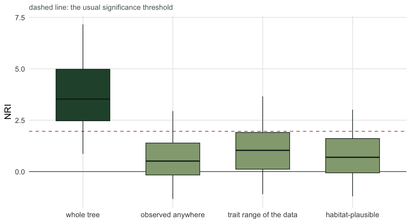
The whole-tree pool gives mean NRI +3.62 and flags 78 per cent of sites. Restricting the pool to species seen somewhere in the matrix, a narrowing most reviewers would call conservative and sensible, gives +0.56 and 10 per cent. The other two narrowings give +1.03 with 22 per cent and +0.71 with 12 per cent. Set those beside the whole-tree row and read the four means and the four flagged shares as one table: the spread across pool definitions is the result, and no single row of it is the answer.
Note what did not happen: the data did not change, the tree did not change, the filtering process is exactly as real under every row. What changed is the question. Against the whole tree the communities get one answer; against the species that actually occur in this landscape they get another. Both answers come from the same data, and only one of them is usually reported.
The sweep is three lines. Run it, put the table in your supplement, and if the sign or the significance moves, that is your result: the answer depends on a pool you cannot observe.
Check 2: run your own pipeline on nothing
Before blaming the statistic for check 1, find out whether the statistic works. Feed the pipeline data with no signal at all and count how often it cries wolf. If the standardised effect size behaves, five per cent of null communities should cross the threshold.
set.seed(12); fp15 <- replicate(400, abs(nri(sample(pool, 15), pool)) > 1.96)
set.seed(13); fp5  <- replicate(400, abs(nri(sample(pool,  5), pool)) > 1.96)
set.seed(14); z15  <- replicate(400, nri(sample(pool, 15), pool))

c(false_positive_k15 = mean(fp15), false_positive_k5 = mean(fp5),
  null_mean = mean(z15), null_sd = sd(z15))
false_positive_k15 false_positive_k5 null_mean null_sd
0.05250000 0.06250000 0.01538244 0.97700793 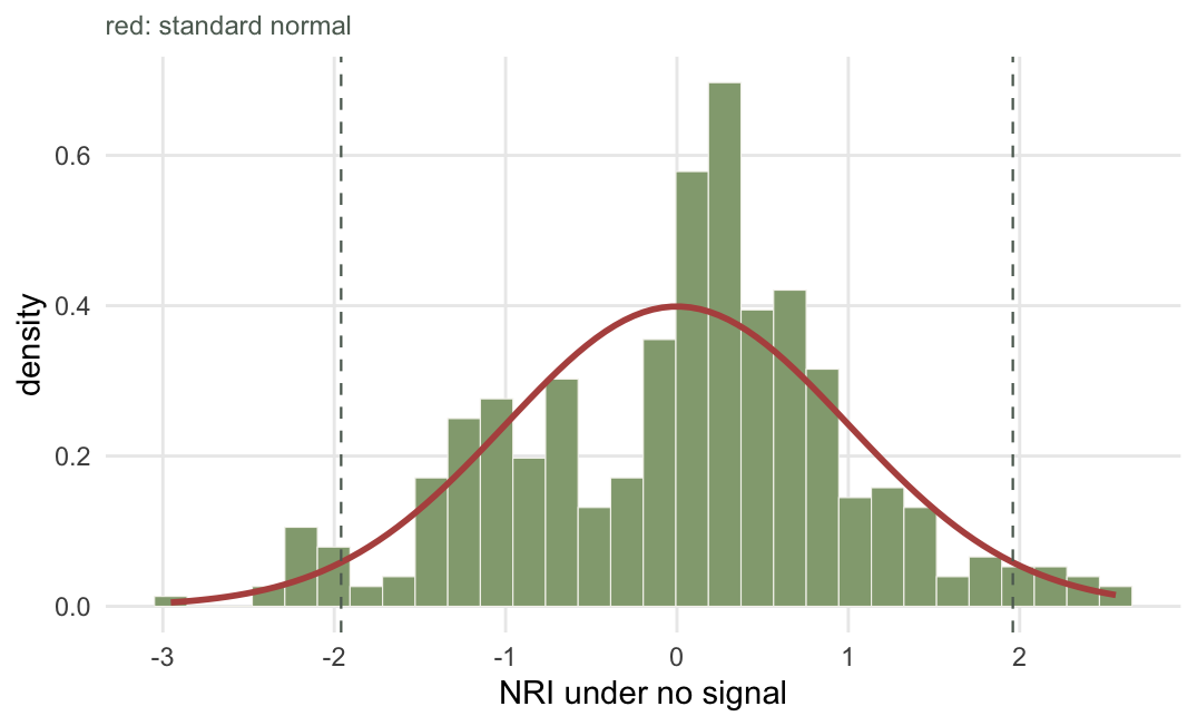
5.2 per cent at fifteen species, 6.2 per cent at five, against a nominal five. The null distribution has mean +0.02 and standard deviation 0.98, close to the standard normal the 1.96 threshold assumes. Each rate rests on 400 replicates, so read them as rough. What went wrong in check 1 was the pool answering a different question, exactly as instructed.
This check costs almost nothing and it is worth doing on your own data rather than trusting this post, because your pipeline is not this pipeline. If the rate comes back well away from the nominal five, the usual cause is a null draw that does not match the observed richness.
Check 3: break the branch lengths
Most community phylogenies are not estimated from your species. They are a published backbone with your taxa grafted on, polytomies resolved by hand, and branch lengths supplied by a rule. Ask what that costs by running the analysis on a tree that keeps the topology and throws the branch lengths away.
tr2 <- tr
tr2$edge.length <- rep(1, nrow(tr2$edge))
D2  <- cophenetic(tr2)[pool, pool]

set.seed(15); v_true <- sapply(comms, nri, pl = pool)
set.seed(15); v_eq   <- sapply(comms, nri, pl = pool, Dm = D2)

c(true_mean = mean(v_true), equal_mean = mean(v_eq),
  true_pct = mean(abs(v_true) > 1.96), equal_pct = mean(abs(v_eq) > 1.96),
  correlation = cor(v_true, v_eq))
true_mean equal_mean true_pct equal_pct correlation
3.5744651 1.3774118 0.7750000 0.2750000 0.4814676 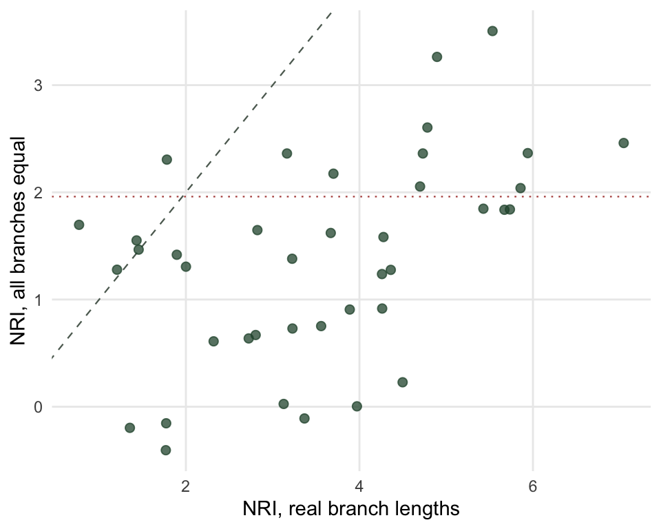
Mean NRI moves from +3.57 to +1.38, and the share of sites flagged from 78 to 28 per cent. Site by site, the two versions correlate at 0.48. That correlation is the check: it is what a reader needs in order to know how much of your result the branch lengths are carrying.
Equal branch lengths are an extreme, and a useful stress test for a tree whose lengths came from a rule rather than from data, but they are not a bound: a different rule can push the answer past the real tree in the other direction. If your tree is dated at the family level and interpolated below, rerun the check with each rule you could have used, because nothing in the output will tell you how much the interpolation moved the answer.
What to report
The three checks fit in one supplementary table and four sentences of methods:
- Which pool, why that pool, and what the sweep across alternatives does to the sign and the significance.
- The false positive rate of your own pipeline on communities you generated with no signal.
- The correlation between your result and the same analysis on a degraded tree.
None of this makes a weak result strong. It makes a strong result believable, and it tells you early when a result is only an artefact of a pool you picked without noticing.
The honest limit
These checks expose the damage from choices you made. They cannot expose the damage from the thing community phylogenetics is actually built on: the assumption that phylogenetic distance stands in for ecological similarity. When that assumption fails, and it fails whenever the traits that matter are convergent or labile, every number in every one of these four posts is precise and about nothing. No amount of checking recovers from that, because the tree cannot tell you it happened. Measuring the traits can.
References
- Cavender-Bares, Kozak, Fine, Kembel 2009 Ecology Letters 12(7):693-715 (10.1111/j.1461-0248.2009.01314.x)
- Swenson 2009 PLoS ONE 4(2):e4390 (10.1371/journal.pone.0004390)
- Kembel, Cowan, Helmus, Cornwell, Morlon, Ackerly, Blomberg, Webb 2010 Bioinformatics 26(11):1463-1464 (10.1093/bioinformatics/btq166)
- Lessard, Borregaard, Fordyce, Rahbek, Weiser, Dunn, Sanders 2012 Proceedings of the Royal Society B 279(1727):266-274 (10.1098/rspb.2011.0552)