library(ape)
library(nlme)
library(ggplot2)

te_paper <- "#f5f4ee"; te_ink   <- "#16241d"; te_body <- "#2c3a31"
te_faint <- "#5d6b61"; te_sage  <- "#93a87f"; te_rust <- "#b5534e"
te_line  <- "#dad9ca"; te_low   <- "#c9b458"; te_high <- "#1d5b4e"

theme_te <- function(base_size = 12) {
  theme_minimal(base_size = base_size) +
    theme(
      plot.background  = element_rect(fill = te_paper, colour = NA),
      panel.background = element_rect(fill = te_paper, colour = NA),
      panel.grid.major = element_line(colour = te_line, linewidth = 0.3),
      panel.grid.minor = element_blank(),
      axis.text  = element_text(colour = te_body),
      axis.title = element_text(colour = te_ink),
      plot.title = element_text(colour = te_ink, face = "bold"),
      strip.text = element_text(colour = te_ink, face = "bold")
    )
}Phylogenetic signal: Blomberg’s K and Pagel’s lambda
R
ape
nlme
phylogenetics
comparative methods
ecology tutorial
Measure phylogenetic signal in species traits with Blomberg’s K and Pagel’s lambda in R: fit both indices, test them against a null, and read the outcome.
Corrected 25 September 2026: the paragraph on tip values filled in from the tree now carries its own measurement. The tree fill does inflate K, but the earlier claim that it can reverse the signal did not survive the simulation.
Closely related species tend to resemble one another, because they share ancestry and have had less time to diverge. Before you run any comparative analysis it helps to ask a prior question: does a trait carry phylogenetic signal at all, and how strong is it? Two indices dominate the literature, and you can compute both in R with ape and nlme alone.
Pagel’s lambda rescales the internal branches of the tree so that the covariance implied by the phylogeny best matches the trait. Lambda near 1 means the trait evolves as if by Brownian motion along the tree; lambda near 0 means the phylogeny carries no information (a star, where every species is independent). Blomberg’s K compares the variance among species to the variance expected under Brownian motion on that exact tree. K near 1 is Brownian-strength signal, K below 1 is weaker than Brownian, and K above 1 means relatives are even more alike than Brownian motion predicts.
Setup
A tree and two traits
There is no field dataset here: the point is to see each index behave against a trait whose history we control. We simulate one ultrametric tree of 40 species, then evolve two traits on it. The first, standing in for something like log body mass, evolves by Brownian motion (Pagel’s lambda set to 1). The second is a labile trait with only a trace of structure (lambda set to 0.1), the kind of behaviour or habitat preference that turns over quickly.
set.seed(414)
tree <- rcoal(40)
tree$tip.label <- sprintf("sp%02d", 1:40)

# simulate a trait with a given Pagel's lambda: scale off-diagonal covariances
sim_pagel <- function(phy, lambda, sigma2 = 1) {
  V <- vcv(phy); Vl <- V * lambda; diag(Vl) <- diag(V)
  x <- MASS::mvrnorm(1, mu = rep(0, nrow(V)), Sigma = sigma2 * Vl)
  setNames(x, rownames(V))
}
set.seed(2)   ; body_mass    <- sim_pagel(tree, lambda = 1.0)
set.seed(291) ; labile_trait <- sim_pagel(tree, lambda = 0.1)
Blomberg’s K by hand
K has a closed form, so there is no need for an extra package. The recipe: find the phylogenetic mean (a generalised-least-squares mean that weights species by the inverse of the phylogenetic covariance), then take the ratio of the raw variance around that mean to the phylogeny-corrected variance, and divide by the value that ratio would take under Brownian motion.
blomberg_K <- function(x, phy) {
  x  <- x[phy$tip.label]; n <- length(x)
  V  <- vcv(phy); Vi <- solve(V); one <- rep(1, n)
  a  <- as.numeric((t(one) %*% Vi %*% x) / (t(one) %*% Vi %*% one))  # phylo mean
  d  <- x - a
  mse_star <- as.numeric(t(d) %*% d) / (n - 1)          # ignores the tree
  mse_phy  <- as.numeric(t(d) %*% Vi %*% d) / (n - 1)    # corrects for the tree
  expected <- (sum(diag(V)) - n / sum(Vi)) / (n - 1)     # value under Brownian motion
  (mse_star / mse_phy) / expected
}

K_mass   <- blomberg_K(body_mass, tree)
K_labile <- blomberg_K(labile_trait, tree)
c(body_mass = K_mass, labile = K_labile)
body_mass labile
1.1024212 0.0102723 The point estimate on its own does not tell you whether signal is more than you would see by chance. The standard test shuffles trait values across the tips many times and rebuilds the null distribution of K; a value in the far right tail means the observed clustering is unlikely without shared history.
set.seed(303); K_mass_null   <- replicate(999, blomberg_K(setNames(sample(body_mass), tree$tip.label), tree))
set.seed(304); K_labile_null <- replicate(999, blomberg_K(setNames(sample(labile_trait), tree$tip.label), tree))
p_mass   <- (1 + sum(K_mass_null   >= K_mass))   / 1000
p_labile <- (1 + sum(K_labile_null >= K_labile)) / 1000
c(p_mass = p_mass, p_labile = p_labile)
p_mass p_labile
0.001 0.555 Body mass gives K of 1.1 with a randomisation p of 0.001; the labile trait gives K of 0.01 with p of 0.56. The first is Brownian-strength signal and highly unlikely by chance; the second is indistinguishable from a phylogeny-free arrangement.
Pagel’s lambda by maximum likelihood
Lambda has a natural likelihood estimate. Fit an intercept-only generalised least squares model with a corPagel correlation structure and let lambda vary; the fitted lambda is the maximum-likelihood value. To test it, compare against the model with lambda fixed at 0, which for an ultrametric tree is exactly the ordinary model with independent, equal-variance errors (a star phylogeny). Twice the difference in log-likelihood is a likelihood-ratio statistic on one degree of freedom.
est_lambda <- function(x, phy) {
  d  <- data.frame(sp = phy$tip.label, y = x[phy$tip.label])
  m1 <- gls(y ~ 1, data = d, correlation = corPagel(0.3, phy, form = ~sp), method = "ML")
  m0 <- gls(y ~ 1, data = d, method = "ML")                       # lambda = 0 (star)
  lam <- as.numeric(coef(m1$modelStruct$corStruct, unconstrained = FALSE))
  lr  <- as.numeric(2 * (logLik(m1) - logLik(m0)))
  c(lambda = lam, LR = lr, p = pchisq(lr, df = 1, lower.tail = FALSE))
}
round(est_lambda(body_mass, tree), 4)
lambda LR p
1.0005 82.2366 0.0000 round(est_lambda(labile_trait, tree), 4)lambda LR p
0.2156 1.1874 0.2759 Body mass returns lambda of essentially 1 with a likelihood-ratio test that is decisive, matching the K result. The labile trait returns lambda near 0.2, and the likelihood-ratio test does not reject lambda of 0: there is no signal worth acting on. The two indices need not agree to the decimal, because K summarises a variance ratio and lambda summarises a branch-scaling; here they agree on the verdict, which is what matters.
Seeing it on the tree
ramp <- colorRampPalette(c(te_low, te_high))
col_from <- function(v) ramp(100)[as.integer(cut(v, breaks = seq(min(v), max(v), length.out = 101), include.lowest = TRUE))]

op <- par(mfrow = c(1, 2), mar = c(1, 0.5, 2.5, 0.5), bg = te_paper, fg = te_body, col.main = te_ink)
plot(tree, show.tip.label = FALSE, edge.color = te_faint, edge.width = 1.2)
tiplabels(pch = 21, bg = col_from(body_mass[tree$tip.label]), col = te_ink, cex = 1.1)
title(main = sprintf("body mass  (K = %.2f, p = %.3f)", K_mass, p_mass), cex.main = 0.95, font.main = 1)
plot(tree, show.tip.label = FALSE, edge.color = te_faint, edge.width = 1.2)
tiplabels(pch = 21, bg = col_from(labile_trait[tree$tip.label]), col = te_ink, cex = 1.1)
title(main = sprintf("labile trait  (K = %.2f, p = %.2f)", K_labile, p_labile), cex.main = 0.95, font.main = 1)
par(op)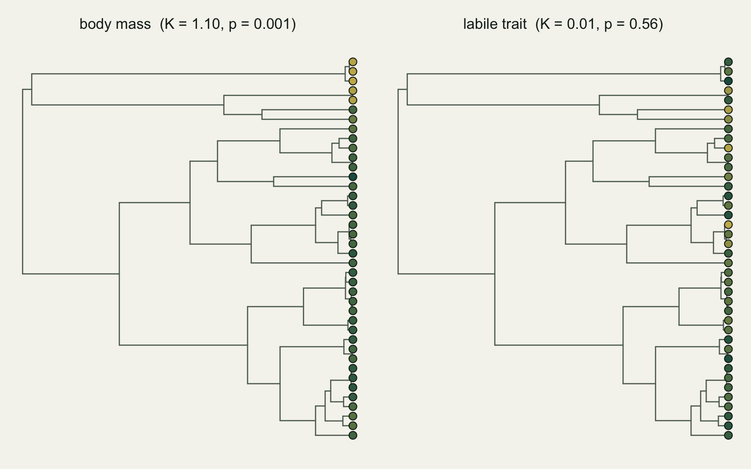
dfn <- rbind(data.frame(trait = "body mass",    K = K_mass_null,   obs = K_mass),
             data.frame(trait = "labile trait", K = K_labile_null, obs = K_labile))
dfn$trait <- factor(dfn$trait, levels = c("body mass", "labile trait"))
ggplot(dfn, aes(K)) +
  geom_histogram(bins = 40, fill = te_sage, colour = te_paper, linewidth = 0.2) +
  geom_vline(aes(xintercept = obs), colour = te_rust, linewidth = 1) +
  facet_wrap(~trait, scales = "free_x") +
  labs(x = "Blomberg's K under tip randomisation", y = "null replicates",
       title = "Observed K (red) against a phylogeny-free null") +
  theme_te(12)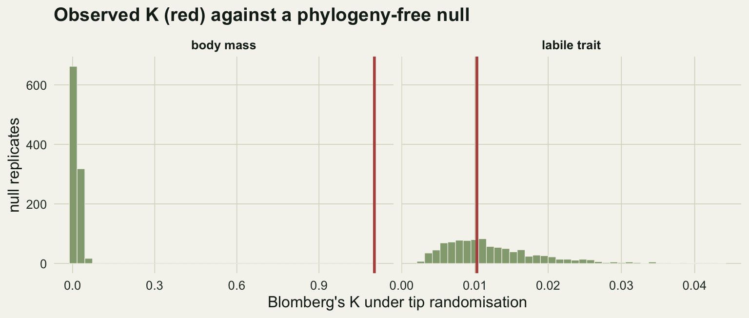
Reading the two indices
Lambda and K answer slightly different questions, and it is worth keeping them apart. Lambda asks how much the branch lengths need to shrink for the phylogeny to explain the trait covariance, and it lives on a natural 0 to 1 scale that many people find easy to report. K asks how the observed variance among species compares to a Brownian expectation, so it can exceed 1 when close relatives are more alike than drift alone would produce, for example under strong niche conservatism. A trait can show a moderate lambda yet a small K, or the reverse, and neither is wrong; they are different summaries.
A few cautions. The point estimate of K from a single trait is noisy: draw a Brownian trait on the same tree a thousand times and K scatters widely around 1, so lean on the test rather than the exact value. Both indices assume the tree and its branch lengths are correct, and error in either propagates into the estimate.
A third source belongs on that list. If any tip value was filled in from the tree rather than measured, the index is partly measuring the fill: predicting a missing tip from its relatives is regression imputation with a phylogeny in place of a fitted line, so the filled tips sit exactly where the model expects them, and the completed matrix conforms to the model more closely than real data ever would. What you report is then not independent of the step that filled the gaps. Filling with the trait mean pushes the estimate the other way, because a constant fill is the same prediction made under an assumed lambda of zero. How far either fill moves the estimate depends on which tips are missing, and the chunk below measures it. It draws 200 fresh 40-species trees for each of four cells: a trait at lambda 1 or 0.5, and tip values lost either as 10 of the 40 drawn at random or as the whole of the one clade whose size is closest to 10 (often exactly 10 tips, otherwise a few more or fewer). Each gap is then filled with the Brownian conditional mean given the measured relatives, filled with the mean of the measured tips, or dropped together with its tip, and K and lambda are compared with their values on the complete data. Lambda comes from a likelihood profile on a grid of 0.02 rather than from gls(), which keeps the chunk fast.
lambda_grid <- function(x, phy) {   # profile likelihood for lambda, grid of 0.02
  V <- vcv(phy)[names(x), names(x)]; n <- length(x); one <- rep(1, n)
  ll <- sapply(seq(0, 1, 0.02), function(l) {
    Vl <- V * l; diag(Vl) <- diag(V); R <- chol(Vl)
    z1 <- backsolve(R, one, transpose = TRUE); zx <- backsolve(R, x, transpose = TRUE)
    a <- sum(z1 * zx) / sum(z1^2); r <- zx - a * z1
    -0.5 * (n * log(sum(r^2) / n) + 2 * sum(log(diag(R))))
  })
  seq(0, 1, 0.02)[which.max(ll)]
}
fill_tree <- function(x, phy, gone) {   # Brownian conditional mean from the measured tips
  V <- vcv(phy)[names(x), names(x)]; keep <- !gone
  Vi <- solve(V[keep, keep]); one <- rep(1, sum(keep))
  a <- as.numeric((one %*% Vi %*% x[keep]) / (one %*% Vi %*% one))
  x[gone] <- a + V[gone, keep] %*% Vi %*% (x[keep] - a); x
}
one_tree <- function(lambda_true, gaps) {
  tr <- rcoal(40); tr$tip.label <- sprintf("sp%02d", 1:40)
  x  <- sim_pagel(tr, lambda = lambda_true)
  if (gaps == "random") {
    gone <- tr$tip.label %in% sample(tr$tip.label, 10)
  } else {
    clades <- prop.part(tr)
    gone <- tr$tip.label %in% tr$tip.label[clades[[which.min(abs(lengths(clades) - 10))]]]
  }
  gone <- setNames(gone, tr$tip.label)[names(x)]
  x_tree <- fill_tree(x, tr, gone)
  x_mean <- x; x_mean[gone] <- mean(x[!gone])
  kept <- drop.tip(tr, names(x)[gone])
  c(K_full = blomberg_K(x, tr), K_tree = blomberg_K(x_tree, tr),
    K_mean = blomberg_K(x_mean, tr), K_drop = blomberg_K(x[!gone], kept),
    L_full = lambda_grid(x, tr), L_tree = lambda_grid(x_tree, tr),
    L_mean = lambda_grid(x_mean, tr), L_drop = lambda_grid(x[!gone], kept))
}
set.seed(163)
n_tree <- 200
cells <- expand.grid(lambda = c(1, 0.5), gaps = c("random", "clade"), stringsAsFactors = FALSE)
runs  <- lapply(seq_len(nrow(cells)), function(i)
  replicate(n_tree, one_tree(cells$lambda[i], cells$gaps[i])))
fills <- do.call(rbind, lapply(seq_len(nrow(cells)), function(i) {
  m <- runs[[i]]
  data.frame(cells[i, ],
             K_tree = median(m["K_tree", ] / m["K_full", ]),
             K_mean = median(m["K_mean", ] / m["K_full", ]),
             K_drop = median(m["K_drop", ] / m["K_full", ]),
             tree_up = mean(m["K_tree", ] > m["K_full", ]),
             lam_full = mean(m["L_full", ]), lam_tree = mean(m["L_tree", ]),
             lam_mean = mean(m["L_mean", ]), lam_drop = mean(m["L_drop", ]))
}))
print(fills, digits = 3, row.names = FALSE)
lambda gaps K_tree K_mean K_drop tree_up lam_full lam_tree lam_mean lam_drop
1.0 random 1.29 0.0925 0.991 0.980 0.999 1.000 0.844 0.998
0.5 random 1.42 0.8743 1.161 0.850 0.326 0.503 0.243 0.311
1.0 clade 1.12 0.9668 1.015 0.660 0.999 0.998 0.999 0.999
0.5 clade 1.00 0.9384 0.988 0.505 0.325 0.370 0.325 0.295cell <- function(l, g) which(fills$lambda == l & fills$gaps == g)
share_se <- sqrt(0.25 / n_tree)
# how many cells each arm keeps within the largest drop-tips miss of the other three
drop_dev <- max(abs(fills$K_drop[-cell(0.5, "random")] - 1))
n_close <- sapply(fills[c("K_tree", "K_mean", "K_drop")], function(r) sum(abs(r - 1) <= drop_dev))
worst_miss <- min(abs(unlist(fills[cell(0.5, "random"), c("K_tree", "K_mean", "K_drop")]) - 1))The K columns are medians over trees of the ratio to the complete-data K, and tree_up is the share of trees in which the tree fill raised K. The tree fill does inflate the index. With the gaps at random its median ratio is 1.29 at lambda 1 and 1.42 at lambda 0.5, and it raises K in 98 and 85 per cent of trees. With one clade missing the inflation shrinks, to 1.12 at lambda 1. An earlier version of this post said that where signal is strong the clade-wise effect can even reverse. The measurement puts it the other way round: it is under the weaker signal that the inflation disappears, with a median ratio of 1.00 at lambda 0.5 and K raised in 50 per cent of trees, while under Brownian signal it still goes up in 66 per cent. No cell reverses in the median (the smallest median ratio of the tree fill is 1.004). The Monte Carlo standard error of each share is at most 3.5 percentage points.
Under Brownian signal with random gaps the mean fill is the larger effect: it cuts K to a median 0.09 of its complete-data value, because the phylogenetic variance in the denominator of K weights differences between close relatives most heavily, and a filled tip differs from a measured sister by that sister’s whole distance from the mean. At lambda 0.5 the same fill gives 0.87. With a whole clade missing it is nearly harmless (0.97 and 0.94), since the filled tips are one another’s closest relatives and agree exactly. Dropping the tips and pruning the tree keeps the median ratio within 0.02 of 1 in three cells; at lambda 0.5 with random gaps it is 1.16, the one cell where even dropping moves K by more than a few per cent. Lambda shows the fills through a different window. At a true lambda of 0.5 the complete-data estimate averages 0.33 on 40 tips, the tree fill with random gaps lifts it to 0.50 and the mean fill lowers it to 0.24: the tree fill lands near the true value only because a quarter of the tips were made to follow a Brownian tree. For K the practical reading is to drop the missing tips rather than fill them before computing the index: dropping stays within that 0.02 of the complete-data K in 3 of the four cells, the tree fill in 1 and the mean fill in 0, and in the fourth cell (lambda 0.5, random gaps) no arm comes closer than 0.13.
Most importantly, signal is a pattern, not a process. A high lambda is consistent with Brownian drift, but also with slow stabilising selection or shared environments among relatives; the index tells you the trait is phylogenetically structured, not why.
If a trait shows signal, the species are not independent data points, and analyses that ignore that will misbehave. That is the starting point for phylogenetic generalised least squares and independent contrasts.
References
- Pagel 1999 Nature 401:877-884 (10.1038/44766)
- Blomberg, Garland & Ives 2003 Evolution 57(4):717-745 (10.1111/j.0014-3820.2003.tb00285.x)
- Freckleton, Harvey & Pagel 2002 The American Naturalist 160(6):712-726 (10.1086/343873)
- Revell, Harmon & Collar 2008 Systematic Biology 57(4):591-601 (10.1080/10635150802302427)
- Munkemuller et al. 2012 Methods in Ecology and Evolution 3(4):743-756 (10.1111/j.2041-210X.2012.00196.x)
- Paradis & Schliep 2019 Bioinformatics 35(3):526-528 (10.1093/bioinformatics/bty633)