Ancestral state reconstruction in R

Ancestral state reconstruction in R with ape: fitting continuous and discrete trait models with ace, reading node uncertainty, and when not to trust it.

Ancestral state reconstruction asks what a trait looked like at the internal nodes of a phylogeny: the value carried by a common ancestor, inferred from the values measured in its living descendants. It is how comparative biologists put numbers on the past, whether that past is the body size of an ancestral finch or the habitat a lineage occupied before it diversified. The estimate is always a model-based guess, and the honest form of the answer carries an interval around it. This post fits one continuous and one discrete reconstruction in R with ape, and spends as much attention on the uncertainty as on the point estimate.

Reconstructing a continuous trait

For a continuous trait the usual model is Brownian motion: the trait drifts up or down at random along every branch, with variance proportional to time. ace fits this by maximum likelihood and returns an estimate at every internal node, each with a 95% confidence interval. We simulate a trait on a forty-tip tree with a true root value of zero, then ask the method to recover it.

library(ape)
library(ggplot2)

te_paper <- "#f5f4ee"; te_ink   <- "#16241d"; te_body <- "#2c3a31"
te_faint <- "#5d6b61"; te_sage  <- "#93a87f"; te_rust <- "#b5534e"
te_line  <- "#dad9ca"; te_green <- "#2f8f63"; te_gold <- "#cda23f"
te_forest <- "#275139"

theme_te <- function(base_size = 12) {
  theme_minimal(base_size = base_size) +
    theme(
      plot.background  = element_rect(fill = te_paper, colour = NA),
      panel.background = element_rect(fill = te_paper, colour = NA),
      panel.grid.major = element_line(colour = te_line, linewidth = 0.3),
      panel.grid.minor = element_blank(),
      axis.text  = element_text(colour = te_body),
      axis.title = element_text(colour = te_ink),
      plot.title = element_text(colour = te_ink, face = "bold"),
      strip.text = element_text(colour = te_ink, face = "bold")
    )
}

set.seed(7)
tr_c <- rcoal(40)
tr_c$tip.label <- sprintf("t%02d", 1:40)
set.seed(20)
xc <- rTraitCont(tr_c, model = "BM", sigma = 1, root.value = 0)  # true root = 0

fit_c <- ace(xc[tr_c$tip.label], tr_c, type = "continuous", method = "ML")
root_est <- fit_c$ace[1]        # first internal node is the root
root_ci  <- fit_c$CI95[1, ]
c(root_estimate = root_est, lower = root_ci[1], upper = root_ci[2])

root_estimate.41            lower            upper 
      0.01210844      -0.77879659       0.80301347 

The reconstructed root value is 0.01, essentially the true zero. That looks like a triumph until you read the interval beside it: the 95% CI runs from -0.78 to 0.8, a span of 1.58 trait units, which is wider than most of the spread among the living species. The point estimate is good here by luck of the draw; the interval is the part you should quote. A single realisation of Brownian motion drifts freely, so the root is only ever pinned down loosely, and a reconstruction reported without its interval hides exactly how loose that is.

The interval also grows with depth. Nodes near the tips sit close to a couple of measured species and inherit tight bounds; the root sits behind hundreds of thousands of generations of possible drift and gets the widest bound of all.

Ntip <- length(tr_c$tip.label)
nn   <- (Ntip + 1):(Ntip + tr_c$Nnode)
bt   <- branching.times(tr_c)
dfc  <- data.frame(node = nn, age = as.numeric(bt[as.character(nn)]),
                   est = fit_c$ace, lo = fit_c$CI95[, 1], hi = fit_c$CI95[, 2])
dfc$root <- dfc$node == (Ntip + 1)
ggplot(dfc, aes(age, est)) +
  geom_hline(yintercept = 0, colour = te_faint, linetype = "22") +
  geom_linerange(aes(ymin = lo, ymax = hi, colour = root), linewidth = 0.6, alpha = 0.8) +
  geom_point(aes(colour = root), size = 1.8) +
  scale_colour_manual(values = c(`FALSE` = te_sage, `TRUE` = te_rust), guide = "none") +
  scale_x_reverse() +
  annotate("text", x = max(dfc$age), y = dfc$est[dfc$root] + 0.18, label = "root",
           colour = te_rust, hjust = 0, size = 3.5, fontface = "bold") +
  labs(x = "node age (time before present)", y = "reconstructed trait value",
       title = "Uncertainty grows toward the root") +
  theme_te(12)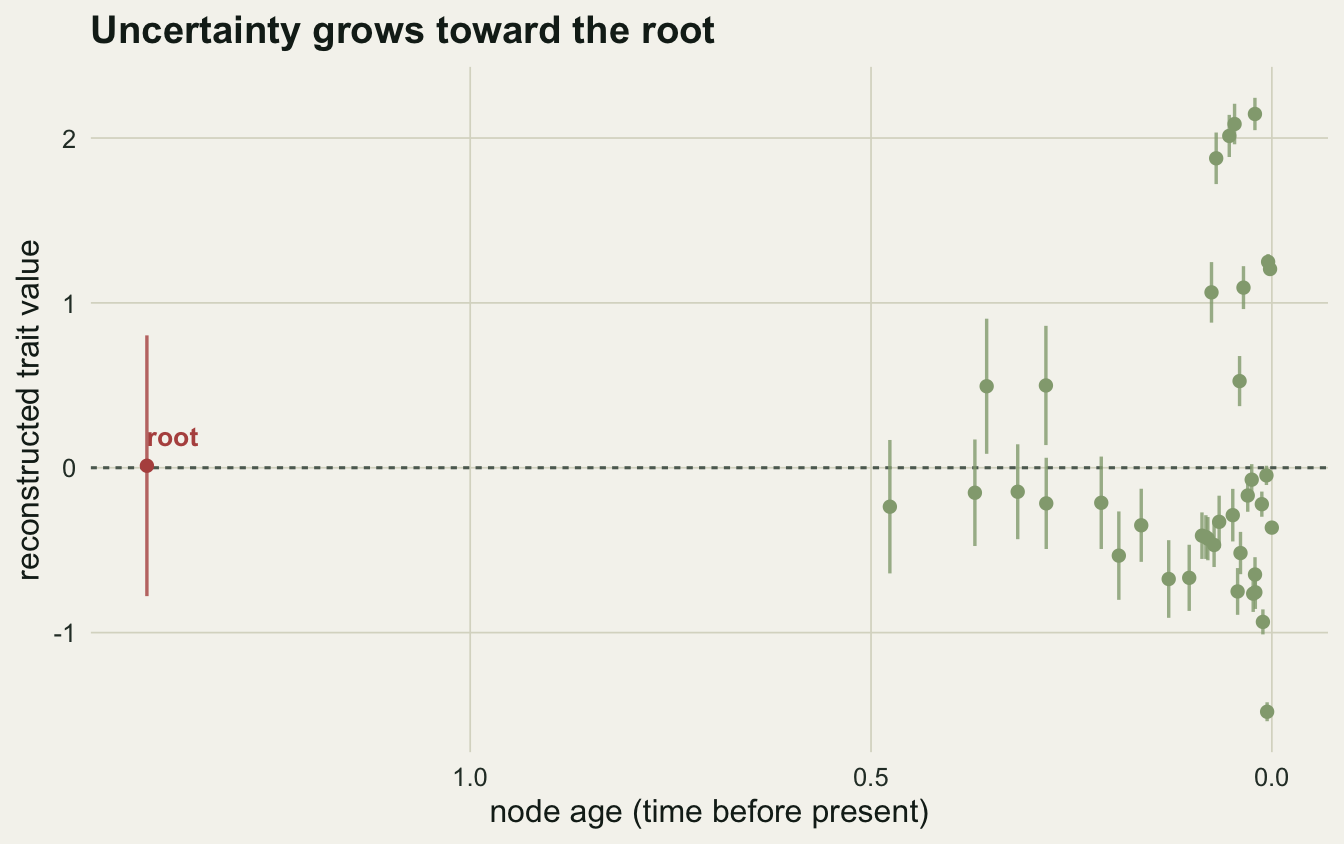

Figure 1: Reconstructed values with 95% confidence intervals for every internal node, plotted against node age. Shallow nodes near the present are pinned tightly by nearby tips; the root (in rust) carries the widest interval. The dashed line marks the true root value of zero.

Reconstructing a discrete trait

Discrete traits, such as a habitat coded as open or forest, use a continuous-time Markov model instead. The simplest version, the equal-rates or ER model, allows changes in either direction at one shared rate. ace estimates that rate and returns, for every node, the scaled likelihood of each state: a probability that the ancestor was open rather than forest. We simulate a two-state habitat on a thirty-six-tip tree and reconstruct it.

set.seed(58)
tr_d <- rcoal(36)
tr_d$tip.label <- sprintf("s%02d", 1:36)
set.seed(58)
xd <- rTraitDisc(tr_d, model = "ER", k = 2, rate = 0.6,
                 states = c("open", "forest"), root.value = 1)

Warning in rTraitDisc(tr_d, model = "ER", k = 2, rate = 0.6, states = c("open",
: package expm not available, using ape::matexpo instead

tb <- table(factor(xd, levels = c("open", "forest")))

fit_d <- ace(xd[tr_d$tip.label], tr_d, type = "discrete", model = "ER")
rootp <- fit_d$lik.anc[1, ]           # state probabilities at the root
c(rate = unname(fit_d$rates), rootp)

     rate      open    forest 
0.2194242 0.8065936 0.1934064 

The tips split 16 open and 20 forest, and the estimated transition rate is 0.22. At the root the model puts 81% of the probability on open and 19% on forest. That is a real answer, and a useful one, but it is not certainty: roughly one time in five the root was forest, on this model and this tree. Reporting only “the ancestor was open” would throw away that caveat.

The picture is not uniformly uncertain, though. Nodes close to the tips, where descendants agree, are reconstructed with near-total confidence; the doubt concentrates in the deep nodes, where competing histories are hard to tell apart.

co <- c(open = te_gold, forest = te_forest)
par(bg = te_paper, mar = c(0, 0, 2, 0))
plot(tr_d, show.tip.label = FALSE, edge.color = te_faint, edge.width = 1.3)
title(main = "Confident tips, uncertain deep nodes", col.main = te_ink,
      cex.main = 1.0, font.main = 2)
tiplabels(pch = 21, bg = co[as.character(xd[tr_d$tip.label])], col = te_paper, cex = 1.2)
nodelabels(pie = fit_d$lik.anc, piecol = c(te_gold, te_forest), cex = 0.45)
legend("bottomleft", legend = c("open", "forest"), pt.bg = c(te_gold, te_forest),
       pch = 21, col = te_paper, bty = "n", text.col = te_body, cex = 0.9)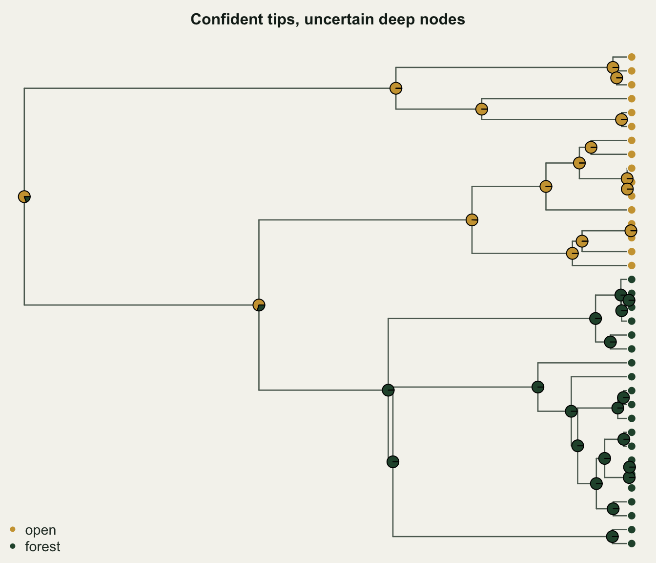

Figure 2: The reconstructed habitat across the tree. Tip circles show the observed state; node pies show the probability of open (gold) against forest (green). The open and forest clades resolve confidently, while the deepest nodes, including the root, keep a visible minority slice.

How much to trust it

A reconstruction is a statement about a model, not a memory of the past, and three limits follow from that. The estimate depends on the model you chose: Brownian motion assumes no trend, so if the trait was under directional selection the reconstructed root will be pulled toward the modern mean and mislead you. A single trait carries limited information about deep history, which is why the root interval was so wide and the deep habitat pies stayed mixed; adding more tips helps near the tips but does little for the root. And a point estimate on its own is close to meaningless here, because the whole value of the method is in the interval or the probability it reports alongside.

Used with that in mind, ace is a clear way to see both what the data suggest about the past and how firmly they suggest it. When the intervals are narrow the reconstruction is worth leaning on; when they are wide, as at a deep root, the right conclusion is often that the trait’s early history is simply not recoverable from living species alone. For questions about correlated change between traits, a method that tests the pattern directly, without committing to reconstructed ancestors, is usually the safer tool, and the tree-aware regression in phylogenetic generalised least squares is one such route.

References

• Felsenstein 1985 The American Naturalist 125(1):1-15 (10.1086/284325)
• Schluter et al 1997 Evolution 51(6):1699-1711 (10.1111/j.1558-5646.1997.tb05095.x)
• Pagel 1994 Proceedings of the Royal Society B 255(1342):37-45 (10.1098/rspb.1994.0006)
• Paradis & Schliep 2019 Bioinformatics 35(3):526-528 (10.1093/bioinformatics/bty633)

Related tutorials

• Phylogenetic signal: Blomberg’s K and Pagel’s lambda
• Independent contrasts: Felsenstein’s method
• Phylogenetic generalised least squares
• Phylogenetic diversity with picante