library(ggplot2)

te_paper  <- "#f5f4ee"
te_ink    <- "#16241d"
te_body   <- "#2c3a31"
te_forest <- "#275139"
te_rust   <- "#b5534e"
te_gold   <- "#c9b458"
te_line   <- "#dad9ca"

theme_datasheet <- function() {
  theme_minimal(base_size = 12) +
    theme(plot.background  = element_rect(fill = te_paper, colour = NA),
          panel.background = element_rect(fill = te_paper, colour = NA),
          panel.grid.major = element_line(colour = te_line, linewidth = 0.3),
          panel.grid.minor = element_blank(),
          text             = element_text(colour = te_body),
          plot.title       = element_text(colour = te_ink, face = "bold"),
          plot.subtitle    = element_text(colour = te_body),
          axis.text        = element_text(colour = te_body))
}Brownian motion or Ornstein-Uhlenbeck?
R
phylogenetics
comparative methods
model selection
simulation
ecology tutorial
Brownian traits on a phylogeny pick an Ornstein-Uhlenbeck model by AICc in about one dataset in seven, bigger trees or not; tip error makes it worse. In R.
Fifty species of lacertid lizard, one dated tree, and a critical thermal maximum measured for each species. The analysis that follows is now routine: fit a Brownian motion model and an Ornstein-Uhlenbeck model to the trait, compare them by AICc, and report the winner. The Ornstein-Uhlenbeck model wins by a few units. The discussion then says that thermal tolerance evolves under stabilising selection towards an optimum, quotes a phylogenetic half-life of about a third of the tree height, and moves on to what the optimum might be.
Every step of that is a standard analysis, and the conclusion is the part that needs checking. An Ornstein-Uhlenbeck model has one parameter more than Brownian motion, a pull of strength alpha towards an optimum, and the question this post measures is how often that extra parameter wins when there was never any pull at all: when the trait was simulated by pure Brownian motion on the very tree used to fit it. It then asks what the fitted alpha of those false wins looks like, whether a real pull can be told apart from a false one by its size, and what a small amount of unmodelled measurement error at the tips does to the comparison.
The site has come close to this question twice without asking it. Phylogenetic generalised least squares compares ordinary regression, corBrownian and corPagel by AIC and recommends letting Pagel’s lambda float. Every model in that comparison is a transformation of one Brownian process: lambda shrinks the shared branch lengths, and nothing in it pulls a trait anywhere. The Ornstein-Uhlenbeck process is a different process with a different covariance, and the comparison here is between processes rather than between rescalings of one tree. Phylogenetic signal: Blomberg’s K and Pagel’s lambda states the confound in one sentence, that a high lambda is consistent with Brownian drift but also with slow stabilising selection, and leaves it there. This post puts a rate on the reverse error: stabilising selection read into data that drifted.
No package for comparative methods is used. The tree is simulated in base R in the way the animal model does it in its section on handing the same code a phylogeny, with one change to the waiting times that is described below, and both models are fitted by profile likelihood with chol and optimize.
Two processes on one tree
Brownian motion on a tree gives each tip a normal value whose covariance with another tip is the length of the path the two share from the root, times the rate sigma squared. With the tree height scaled to one, the diagonal of that matrix is one and the off-diagonal entries are the shared paths. An Ornstein-Uhlenbeck process adds a pull: the trait drifts as before, but it is also drawn back towards an optimum theta at a rate proportional to its distance from it. Hansen brought this process into comparative biology in 1997, and Butler and King wrote out the likelihood fits in 2004.
The covariance depends on what is assumed about the root. The version used throughout this post fixes the root state at the optimum, so every tip has the same expected value and the only difference from Brownian motion is in the covariance. For two tips with shared path s on a tree of height T the fixed-root covariance is sigma squared over 2 alpha, times exp(-2 alpha (T - s)), times (1 - exp(-2 alpha s)). The alternative, a root drawn from the stationary distribution, drops the last factor; it is not used here.
Two tree generators are used, and they differ only in branch lengths. Both work backwards from the tips and merge a uniformly chosen pair of lineages at each step, so both give the same distribution of topologies. In the Yule-like generator the waiting time while k lineages remain is exponential with rate k, which is the interval structure of a pure-birth tree; in the coalescent-like generator the rate is k(k - 1)/2, which crowds most of the merges close to the tips and leaves long branches near the root. The animal model post uses rate k - 1, which is close to the Yule-like case. Either way the result is rescaled to a height of one.
sim_tree <- function(n_tip, shape = c("yule", "coalescent")) {
  shape     <- match.arg(shape)
  clades    <- as.list(seq_len(n_tip))
  split_age <- matrix(0, n_tip, n_tip)
  age <- 0
  k   <- n_tip
  while (k > 1L) {
    rate_k <- if (shape == "yule") k else k * (k - 1) / 2
    age    <- age + rexp(1, rate = rate_k)
    pick   <- sample.int(k, 2)
    g1 <- clades[[pick[1]]]
    g2 <- clades[[pick[2]]]
    split_age[g1, g2] <- age
    split_age[g2, g1] <- age
    clades[[pick[1]]] <- c(g1, g2)
    clades[[pick[2]]] <- NULL
    k <- k - 1L
  }
  shared <- (age - split_age) / age
  diag(shared) <- 1
  shared
}

ou_vcv <- function(shared, alpha) {
  exp(-2 * alpha * (1 - shared)) * (-expm1(-2 * alpha * shared)) / (2 * alpha)
}

set.seed(4127)
tree_demo <- sim_tree(30, "yule")
gap_1e3 <- max(abs(ou_vcv(tree_demo, 1e-3) - tree_demo))
gap_1e6 <- max(abs(ou_vcv(tree_demo, 1e-6) - tree_demo))
As alpha goes to zero the Ornstein-Uhlenbeck covariance should collapse onto the Brownian one, since a process with no pull is Brownian motion. On a 30 tip tree the largest absolute difference between the two matrices is 9.99e-04 at alpha = 0.001 and 1.00e-06 at alpha = 0.000001: the gap shrinks in proportion to alpha, which is what the first-order expansion of the formula predicts.
That check says the formula has the right limit, not that it is right. The second check simulates the process forward, with nothing from the formula in it. On a three-tip tree where tips one and two share a path of 0.6 and tip three splits at the root, an Ornstein-Uhlenbeck path is run along each branch using the exact transition of the process: the value decays by exp(-alpha t) towards the optimum and gains independent normal noise of variance (1 - exp(-2 alpha t)) / (2 alpha).
alpha_chk <- 2
s_node    <- 0.6
n_draw    <- 200000
ou_step <- function(x_from, len, alpha) {
  x_from * exp(-alpha * len) +
    sqrt(-expm1(-2 * alpha * len) / (2 * alpha)) * rnorm(length(x_from))
}
set.seed(8830)
x_node <- ou_step(rep(0, n_draw), s_node, alpha_chk)
x_tip1 <- ou_step(x_node, 1 - s_node, alpha_chk)
x_tip2 <- ou_step(x_node, 1 - s_node, alpha_chk)
x_tip3 <- ou_step(rep(0, n_draw), 1, alpha_chk)
emp_cov <- cov(cbind(x_tip1, x_tip2, x_tip3))
shared_chk <- matrix(c(1, s_node, 0, s_node, 1, 0, 0, 0, 1), 3, 3)
thy_cov <- ou_vcv(shared_chk, alpha_chk)
cov_gap <- max(abs(emp_cov - thy_cov))
cov_se  <- sqrt(2 * max(thy_cov)^2 / n_draw)
With alpha = 2 and 200000 simulated runs of the process on that tree, the empirical covariance of the two sister tips is 0.0454 against 0.0459 from the formula, and the tip variance is 0.2448 against 0.2454. The largest discrepancy across the matrix is 0.0010, against a Monte Carlo standard error of about 0.0008 for a single variance entry. The fixed-root formula is the covariance of the process it claims to describe.
The figure shows what the pull does to the covariance. Brownian motion is a straight line through the origin. A weak pull bends it down a little; a strong one leaves pairs of tips almost uncorrelated unless they split very recently. The data can only see alpha through that bend.
alpha_show <- c(0.25, 1, 4)
s_seq <- seq(0, 1, length.out = 101)
cov_df <- rbind(
  data.frame(s = s_seq, v = s_seq, model = "Brownian motion"),
  do.call(rbind, lapply(alpha_show, function(a_val) {
    data.frame(s = s_seq, v = ou_vcv(s_seq, a_val),
               model = sprintf("OU, alpha = %g", a_val))
  })))
cov_df$model <- factor(cov_df$model, levels = unique(cov_df$model))
ggplot(cov_df, aes(s, v, colour = model)) +
  geom_line(linewidth = 0.9) +
  scale_colour_manual(values = c(te_ink, te_forest, te_gold, te_rust), name = NULL) +
  labs(x = "shared path from the root (tree height = 1)",
       y = "covariance of the two tips",
       title = "The pull flattens the covariance",
       subtitle = "sigma squared = 1, fixed root at the optimum") +
  theme_datasheet() +
  theme(legend.position = "bottom")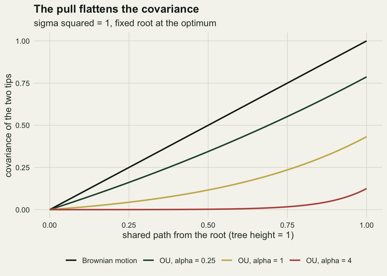
Fitting both models by profile likelihood
Both models have a mean and a rate that can be profiled out exactly. For a fixed correlation matrix R, the generalised least squares mean and the maximum likelihood sigma squared have closed forms, so the log-likelihood of Brownian motion is one Cholesky factorisation and the log-likelihood of the Ornstein-Uhlenbeck model is a function of alpha alone. Brownian motion therefore has two parameters, the mean and sigma squared, and the Ornstein-Uhlenbeck model has three, the same two plus alpha. With the root fixed at the optimum, theta and the root state are the same parameter, which is why the count is three and not four.
AICc is computed with those counts, using the small-sample correction of Hurvich and Tsai, and the Ornstein-Uhlenbeck model is recorded as chosen when its AICc is lower.
alpha_min <- 1e-3
alpha_max <- log(2) / 0.01
n_coarse  <- 20

prof_ll <- function(y, r_mat) {
  n_obs <- length(y)
  ch  <- chol(r_mat)
  y_w <- backsolve(ch, y, transpose = TRUE)
  o_w <- backsolve(ch, rep(1, n_obs), transpose = TRUE)
  mu_hat <- sum(o_w * y_w) / sum(o_w^2)
  s2_hat <- sum((y_w - mu_hat * o_w)^2) / n_obs
  -n_obs / 2 * (log(2 * pi * s2_hat) + 1) - sum(log(diag(ch)))
}

aicc <- function(loglik, n_par, n_obs) {
  -2 * loglik + 2 * n_par + 2 * n_par * (n_par + 1) / (n_obs - n_par - 1)
}

fit_bm_ou <- function(y, shared) {
  n_obs <- length(y)
  ll_bm <- prof_ll(y, shared)
  ll_a  <- function(log_a) prof_ll(y, ou_vcv(shared, exp(log_a)))
  la_grid <- seq(log(alpha_min), log(alpha_max), length.out = n_coarse)
  ll_grid <- vapply(la_grid, ll_a, 0)
  i_best  <- which.max(ll_grid)
  bracket <- la_grid[c(max(1, i_best - 1), min(n_coarse, i_best + 1))]
  opt <- optimize(ll_a, bracket, maximum = TRUE)
  if (opt$objective < ll_grid[i_best]) {
    opt <- list(maximum = la_grid[i_best], objective = ll_grid[i_best])
  }
  c(ll_bm = ll_bm, ll_ou = opt$objective, alpha = exp(opt$maximum),
    pick_ou = aicc(opt$objective, 3, n_obs) < aicc(ll_bm, 2, n_obs))
}

sim_fit <- function(n_tip, n_rep, shape = "yule", alpha_true = 0, me_var = 0) {
  out <- t(replicate(n_rep, {
    shared <- sim_tree(n_tip, shape)
    v_true <- if (alpha_true == 0) shared else ou_vcv(shared, alpha_true)
    y <- drop(crossprod(chol(v_true), rnorm(n_tip))) + rnorm(n_tip, 0, sqrt(me_var))
    fit_bm_ou(y, shared)
  }))
  as.data.frame(out)
}

set.seed(5511)
one_fit <- fit_bm_ou(drop(crossprod(chol(tree_demo), rnorm(30))), tree_demo)
Alpha is searched on the log scale between 0.001, which is Brownian motion to three decimal places in the covariance, and 69.3, which is a half-life of one hundredth of the tree height. A coarse grid of 20 values finds the best bracket and optimize refines inside it, because optimize assumes a single maximum inside its interval and the grid is the cheap guard against a profile with more than one.
On one Brownian dataset simulated on the demonstration tree, the Brownian log-likelihood is -27.914 and the best Ornstein-Uhlenbeck log-likelihood is -27.914, with alpha at 0.001, the lower bound. That is what the boundary looks like from inside the fit: the extra parameter is not wanted, it goes as close to zero as the search allows, and the two likelihoods agree to three decimal places. The deficit of 0.0004 on the Ornstein-Uhlenbeck side is the cost of stopping at alpha = 0.001 rather than at zero, and it cannot make the model win.
How often Brownian data choose OU
The design was fixed before the simulation ran: 25, 50 and 100 tips, a fresh tree for every dataset, 1000 Brownian datasets per tree size on Yule-like trees and 500 on coalescent-like trees. There is a textbook benchmark to set the rates against, with a caveat that comes up below. Self and Liang give the large-sample distribution of the likelihood ratio when the null value of a parameter sits on the edge of its range: half the time the estimate is on the boundary and the statistic is zero, and the other half it behaves like a chi-squared with one degree of freedom. That result assumes the information about the parameter keeps growing with the sample.
tip_grid <- c(25, 50, 100)
n_rep_bm <- 1000
n_rep_sh <- 500

set.seed(20260825)
null_yule <- lapply(tip_grid, function(n_tip) sim_fit(n_tip, n_rep_bm, "yule"))
set.seed(20260826)
null_coal <- lapply(tip_grid, function(n_tip) sim_fit(n_tip, n_rep_sh, "coalescent"))

rate_tab <- function(fits, lab) {
  p_hat <- vapply(fits, function(f) mean(f$pick_ou), 0)
  n_r   <- vapply(fits, nrow, 0)
  data.frame(n_tip = tip_grid, rate = p_hat,
             se = sqrt(p_hat * (1 - p_hat) / n_r), tree = lab)
}
rates_null <- rbind(rate_tab(null_yule, "Yule-like tree"),
                    rate_tab(null_coal, "coalescent-like tree"))

chibar_rate <- vapply(tip_grid, function(n_tip) {
  lr_cut <- aicc(0, 3, n_tip) - aicc(0, 2, n_tip)
  0.5 * pchisq(lr_cut, df = 1, lower.tail = FALSE)
}, 0)
lr_cut_25 <- aicc(0, 3, 25) - aicc(0, 2, 25)

ry  <- rates_null[rates_null$tree == "Yule-like tree", ]
rc  <- rates_null[rates_null$tree == "coalescent-like tree", ]
ratio_y <- ry$rate / chibar_rate
diff_y  <- ry$rate[3] - ry$rate[1]
diff_se <- sqrt(ry$se[3]^2 + ry$se[1]^2)
ratio_c <- rc$rate / ry$rate
at_floor <- vapply(null_yule, function(f) mean(f$alpha < alpha_min * 1.01), 0)
at_ceil  <- vapply(null_yule, function(f) mean(f$alpha > alpha_max * 0.99), 0)
interior <- 1 - at_floor
AICc prefers the Ornstein-Uhlenbeck model when twice the log-likelihood gain exceeds the difference in penalties, which is 2.60 at 25 tips, so the benchmark rate is half the chi-squared tail above that cut.
On Yule-like trees AICc chose the Ornstein-Uhlenbeck model for 13.7, 14.2 and 14.1 per cent of Brownian datasets at 25, 50 and 100 tips, each with a Monte Carlo standard error of 1.1 percentage points or less. The boundary benchmark predicts 5.4, 6.6 and 7.2 per cent, so the measured rate is between 1.9 and 2.6 times the benchmark value. The benchmark assumes information about alpha keeps growing with the sample, which on a tree of fixed height it does not (Ho and Ane, below), so the gap measures how far this setting is from textbook asymptotics rather than a failure of the theory.
The rate does not fall with more tips. The difference between 100 and 25 tips is +0.4 percentage points with a standard error of 1.5, which is no measurable change. Quadrupling the number of species did not measurably change the chance of inventing a pull. Ho and Ane show that maximum likelihood estimates of Ornstein-Uhlenbeck parameters can be inaccurate and even non-unique when only present-day species are observed, and that the problem is a property of such trees rather than of small samples. A plausible mechanism for the flat rate here is that on a tree of fixed height the added tips mostly split recently, so they add little information about a covariance that bends over the depth of the tree.
Tree shape changed the rate where tree size did not. On coalescent-like trees the rates were 22.8, 25.4 and 27.8 per cent, between 1.7 and 2.0 times the Yule-like rates at the same size. Those trees have most of their splits packed near the tips and a few long branches from the root, and a plausible reading is that a Brownian dataset on them carries even less information about how the covariance bends with shared path.
The boundary share is a second sign that the asymptotics do not apply here. The benchmark has alpha on its lower bound in half of the datasets. On Yule-like trees it was on the bound in 29.3, 33.6 and 39.0 per cent, so the interior estimates that feed the false picks were between 61.0 and 70.7 per cent of fits instead of one half. No fit ended on the upper bound of 69.3: the largest share at the ceiling across sizes was 0.0 per cent, so the bound did not censor anything.
bench_df <- data.frame(n_tip = tip_grid, rate = chibar_rate)
ggplot(rates_null, aes(n_tip, rate, colour = tree)) +
  geom_line(data = bench_df, aes(n_tip, rate), inherit.aes = FALSE,
            linetype = "dashed", colour = te_body, linewidth = 0.6) +
  geom_errorbar(aes(ymin = rate - 1.96 * se, ymax = rate + 1.96 * se),
                width = 3, linewidth = 0.5) +
  geom_line(linewidth = 0.9) +
  geom_point(size = 2.4) +
  scale_colour_manual(values = c(te_rust, te_forest), name = NULL) +
  scale_x_continuous(breaks = tip_grid) +
  scale_y_continuous(limits = c(0, NA)) +
  labs(x = "number of tips", y = "share of Brownian datasets where AICc picks OU",
       title = "More tips do not cure the false pull",
       subtitle = "dashed: the large-sample boundary benchmark; bars: 95% Monte Carlo intervals") +
  theme_datasheet() +
  theme(legend.position = "bottom")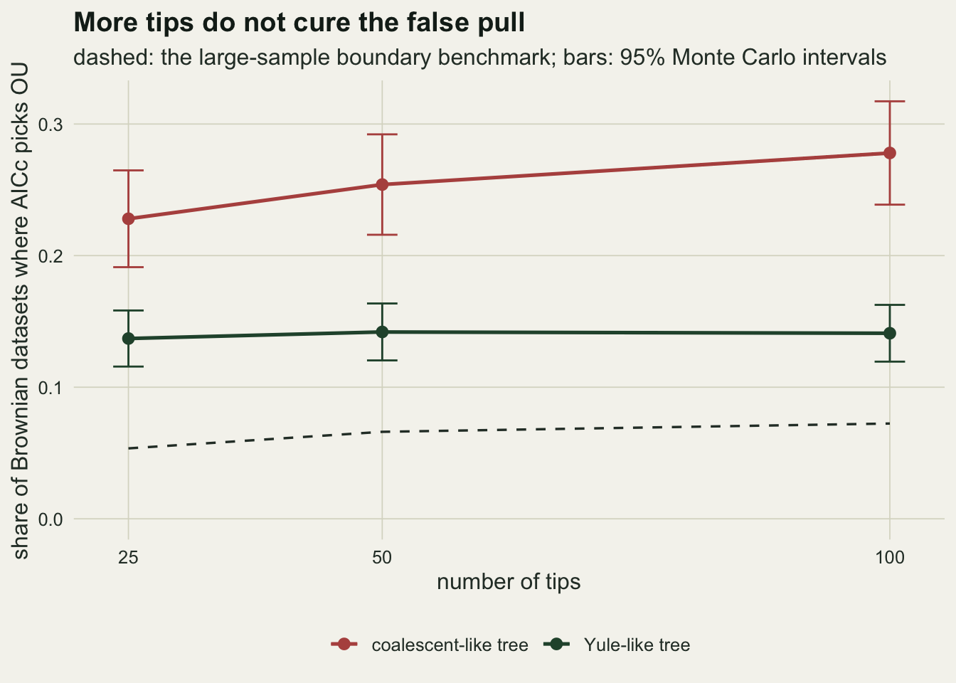
The alpha of a false pick looks like selection
A false pick would be harmless if its alpha were so small that nobody would read it as selection. To see whether it is, the fitted alpha is converted to the phylogenetic half-life, log(2) / alpha, the time for the expected distance from the optimum to halve, in units of tree height. As a positive control the same fits were run on 500 datasets per tree size simulated under a real Ornstein-Uhlenbeck process with a half-life of 0.5, half the tree height, which corresponds to alpha = log(2) / 0.5. That value was chosen before the run as a moderate pull, the kind of number a paper would describe as stabilising selection.
alpha_true <- log(2) / 0.5
set.seed(7731)
pos_yule <- lapply(tip_grid, function(n_tip) sim_fit(n_tip, n_rep_sh, "yule",
                                                     alpha_true = alpha_true))
pos_rate <- vapply(pos_yule, function(f) mean(f$pick_ou), 0)
pos_se   <- sqrt(pos_rate * (1 - pos_rate) / n_rep_sh)


hl_false <- lapply(null_yule, function(f) log(2) / f$alpha[f$pick_ou == 1])
hl_med   <- vapply(hl_false, median, 0)
hl_below <- vapply(hl_false, function(h) mean(h < 1), 0)
hl_true  <- lapply(pos_yule, function(f) log(2) / f$alpha[f$pick_ou == 1])
hl_true_med <- vapply(hl_true, median, 0)
i50 <- which(tip_grid == 50)
hl_max_50  <- max(hl_false[[i50]])
hl_half_50 <- mean(hl_false[[i50]] < 0.5)
The median half-life of the false picks on Yule-like trees was 0.28, 0.44 and 0.62 of the tree height at 25, 50 and 100 tips. The share of false picks with a half-life shorter than the whole tree was 100.0, 100.0 and 97.2 per cent. At 50 tips the longest false half-life was 0.77, and 69.0 per cent of them were shorter than 0.5.
This is a selection effect, not a coincidence. A false pick only happens when alpha is large enough to bend the covariance by more than the penalty for one parameter, so every false pick is, by construction, a pull strong enough to be noticed. Small alphas that would read as near-Brownian do not win and never enter the sample of reported results.
The positive control shows why the size of alpha cannot be used to spot the false ones. Real Ornstein-Uhlenbeck data with a half-life of 0.5 were detected in 58.8, 79.2 and 92.6 per cent of datasets, with standard errors up to 2.2 percentage points, and the median fitted half-life among the detections was 0.24, 0.32 and 0.40: the median fitted pull among detections is too strong, partly because detection itself selects large alphas, and the gap narrows as tips are added. At 50 tips the median half-life was 0.32 for the real detections and 0.44 for the false ones, and the two histograms in the figure overlap across most of their range. A reader given one fitted half-life from that range has no way to tell which process produced it.
hl_df <- rbind(
  data.frame(hl = hl_false[[i50]], source = "Brownian data, OU picked"),
  data.frame(hl = hl_true[[i50]], source = "OU data (half-life 0.5), OU picked"))
ggplot(hl_df, aes(hl, fill = source)) +
  geom_histogram(aes(y = after_stat(density)), bins = 30, position = "identity",
                 alpha = 0.6, colour = NA) +
  geom_vline(xintercept = 0.5, linetype = "dashed", colour = te_ink, linewidth = 0.6) +
  scale_x_log10(breaks = c(0.05, 0.1, 0.2, 0.3, 0.5, 1)) +
  scale_fill_manual(values = c(te_rust, te_forest), name = NULL) +
  labs(x = "fitted phylogenetic half-life, log(2) / alpha (tree height = 1)",
       y = "density",
       title = "False and real pulls overlap in half-life",
       subtitle = "50 tips, Yule-like trees; dashed: the true half-life of the OU data") +
  theme_datasheet() +
  theme(legend.position = "bottom")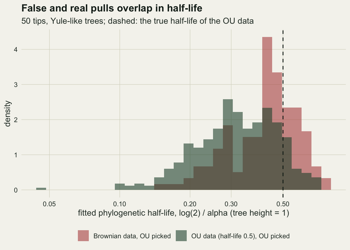
Measurement error manufactures the pull
The last piece is the one that happens in real data. A species mean is estimated from a handful of individuals, and that estimate carries sampling error that is independent between species. Brownian motion has no term for it, so the extra variance sits on the diagonal of the tip covariance and makes every species look a little less like its relatives than the tree predicts. An Ornstein-Uhlenbeck covariance can be written as Brownian motion on the same tree with its terminal branches stretched relative to the internal ones, and independent tip error does exactly that to the terminal branches: both lower the covariance between tips relative to the tip variance, though not by the same pattern across shared paths. The simulation adds independent normal error with variance 0.05 to Brownian data with sigma squared = 1. The level was fixed before the run and not changed afterwards.
me_var <- 0.05
set.seed(3390)
me_yule <- lapply(tip_grid, function(n_tip) sim_fit(n_tip, n_rep_sh, "yule",
                                                    me_var = me_var))
me_rate <- vapply(me_yule, function(f) mean(f$pick_ou), 0)
me_se   <- sqrt(me_rate * (1 - me_rate) / n_rep_sh)
me_hl   <- vapply(me_yule, function(f) median(log(2) / f$alpha[f$pick_ou == 1]), 0)
me_vs_pos <- me_rate - pos_rate
me_share  <- me_var / (1 + me_var)
The error is 4.8 per cent of the total tip variance. With it, AICc chose the Ornstein-Uhlenbeck model for 52.0, 73.6 and 93.2 per cent of datasets at 25, 50 and 100 tips, with standard errors up to 2.2 percentage points. The direction is the opposite of what more data usually does. The error is a real departure from the Brownian model, so the fit gets better at detecting it as tips are added, and the only model on offer that can absorb it is the one with a pull. The median half-life of those picks was 0.21, 0.31 and 0.36.
Set against the positive control, the error-contaminated Brownian data were chosen as Ornstein-Uhlenbeck at rates that differed from those for real Ornstein-Uhlenbeck data with a half-life of 0.5 by -6.8, -5.6 and +0.6 percentage points. Cooper and colleagues made both points from their own simulations: likelihood ratio tests favour Ornstein-Uhlenbeck over simpler models too often, many published datasets are small enough to be exposed to that, and very small amounts of error can change the inference. The numbers here put a rate on both for trees built in a few lines of R, and they show that a small tip error brings pure drift within 6.8 percentage points of a moderate pull at every tree size simulated, as far as AICc is concerned.
me_df <- rbind(
  data.frame(n_tip = tip_grid, rate = ry$rate, se = ry$se,
             data = "Brownian motion"),
  data.frame(n_tip = tip_grid, rate = me_rate, se = me_se,
             data = "Brownian motion + tip error (variance 0.05)"),
  data.frame(n_tip = tip_grid, rate = pos_rate, se = pos_se,
             data = "OU, half-life 0.5"))
ggplot(me_df, aes(n_tip, rate, colour = data)) +
  geom_errorbar(aes(ymin = rate - 1.96 * se, ymax = rate + 1.96 * se),
                width = 3, linewidth = 0.5) +
  geom_line(linewidth = 0.9) +
  geom_point(size = 2.4) +
  scale_colour_manual(values = c(te_ink, te_rust, te_gold), name = NULL) +
  scale_x_continuous(breaks = tip_grid) +
  scale_y_continuous(limits = c(0, 1)) +
  guides(colour = guide_legend(ncol = 1)) +
  labs(x = "number of tips", y = "share of datasets where AICc picks OU",
       title = "Tip error looks like a pull, and more tips make it louder",
       subtitle = "Yule-like trees; bars: 95% Monte Carlo intervals") +
  theme_datasheet() +
  theme(legend.position = "bottom")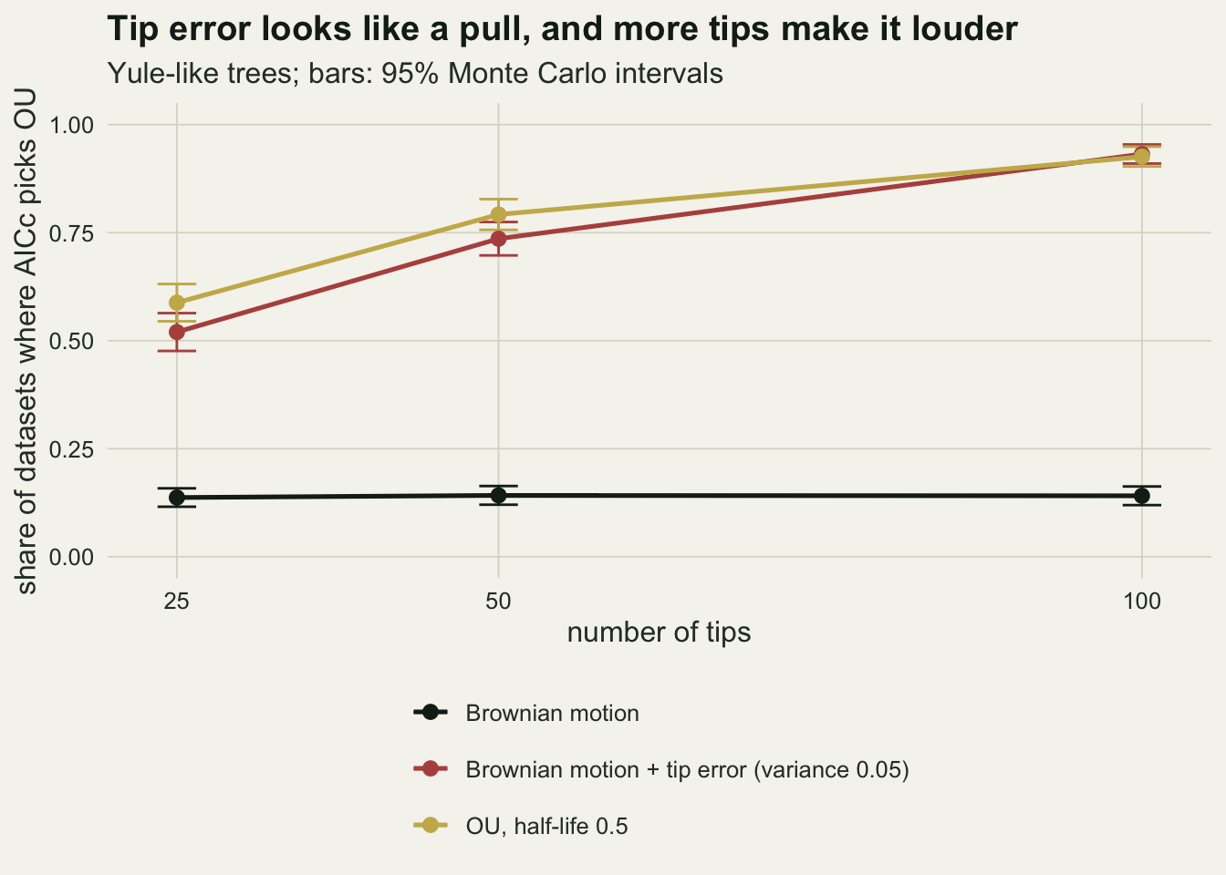
What to report
Report the tree and the size of the comparison before the winner. The number of tips, the tree height in the units used and, if possible, how the tree was dated or simulated, are what a reader needs to judge a model comparison whose error rate depends on tree shape. On the trees simulated here the false choice rate for Ornstein-Uhlenbeck was between 13.7 and 14.2 per cent on Yule-like trees and between 22.8 and 27.8 per cent on coalescent-like trees, and adding species did not bring it down.
Do not treat an AICc difference of a few units as evidence for stabilising selection. The better check is a parametric bootstrap on the tree in hand: simulate Brownian datasets with the fitted Brownian parameters, fit both models to each, and see how often, and by how much, the Ornstein-Uhlenbeck model wins. That gives a calibrated null for the actual tree, which the textbook benchmark cannot provide, and it is the practice Cooper and colleagues recommend: simulate the fitted models and compare the empirical result with the simulations. The same functions in this post do it in a loop.
Give alpha as a half-life with an interval, and say whether the root was fixed at the optimum or drawn from the stationary distribution. A half-life shorter than the tree was the rule among false picks, so a short half-life on its own does not separate selection from drift.
Model the measurement error, or at least say why it was not modelled. If species means were estimated from samples, their standard errors belong on the diagonal of both covariance matrices before the comparison is run. Without that term, an Ornstein-Uhlenbeck win on a tree of a hundred species can come from sampling error as readily as from selection: at a hundred tips in the simulation above, the two gave the same choice rate within Monte Carlo error.
Honest limits
The pull in every simulation acts towards a single optimum equal to the root state. Multiple-optimum models, in which different clades are pulled towards different values, are a common reason to fit Ornstein-Uhlenbeck models in practice, and they add parameters for every optimum. Their false-positive behaviour was not measured here.
The stationary-root variant was not fitted. It changes the covariance of pairs that split near the root, so its false choice rate under Brownian data may differ from the numbers above; the code would need only the last factor of the covariance removed to find out.
The trees are simulated, ultrametric and known without error. Real phylogenies are estimated, their branch lengths are uncertain, and an error in the branch lengths near the tips could produce a pattern like the one measurement error produced here; that was not simulated. The two generators span a balanced-in-time and a tip-crowded shape, and the Ornstein-Uhlenbeck choice rate was higher on the second at every tree size; a tree with long terminal branches, as in a sample of old, species-poor clades, was not simulated and could fall outside that range.
Only one level of tip error and one true alpha were used. The rate at which tip error produces an Ornstein-Uhlenbeck choice was measured at one error size only, and the detection rate of a real pull at one half-life only; the post shows one point of each surface, chosen before the run, and should not be read as a calibration curve.
The grid of tree sizes stops at 100 tips. Larger comparative datasets exist, and the flat false-choice rate is shown only over the fourfold range simulated. The results of Ho and Ane concern the same setting, a tree of fixed height with only present-day species, but the simulation itself does not reach trees of a thousand species, and the flat rate is not shown for them.
References
Hansen TF 1997 Evolution 51(5):1341-1351 (10.1111/j.1558-5646.1997.tb01457.x)
Butler MA, King AA 2004 The American Naturalist 164(6):683-695 (10.1086/426002)
Cooper N, Thomas GH, Venditti C, Meade A, Freckleton RP 2016 Biological Journal of the Linnean Society 118(1):64-77 (10.1111/bij.12701)
Ho LST, Ane C 2014 Methods in Ecology and Evolution 5(11):1133-1146 (10.1111/2041-210X.12285)
Hurvich CM, Tsai CL 1989 Biometrika 76(2):297-307 (10.1093/biomet/76.2.297)
Self SG, Liang KY 1987 Journal of the American Statistical Association 82(398):605-610 (10.1080/01621459.1987.10478472)