library(ggplot2)

te_pal <- list(forest = "#275139", green = "#2f8f63", sage = "#93a87f",
               clay = "#b5534e", gold = "#cda23f", line = "#dad9ca",
               ink = "#16241d", paper = "#f5f4ee")

theme_te <- function() {
  theme_minimal(base_size = 12) +
    theme(panel.grid.minor = element_blank(),
          panel.grid.major = element_line(colour = "#e7e6dc"),
          plot.background = element_rect(fill = "#f5f4ee", colour = NA),
          panel.background = element_rect(fill = "#f5f4ee", colour = NA),
          plot.title = element_text(face = "bold", colour = te_pal$ink),
          axis.title = element_text(colour = "#2c3a31"),
          legend.position = "bottom")
}The animal model in R
R
quantitative genetics
heritability
mixed models
ecology tutorial
Estimate additive genetic variance and narrow-sense heritability from a pedigree in base R: build the relationship matrix, fit REML, predict breeding values.
The ringing team has been opening the same nest boxes every spring for nearly thirty years. Each chick gets a numbered ring before it fledges, and the adult female sitting on the clutch gets caught and read. Over the years that leaves two things in the filing cabinet: a very long list of wing lengths, and a list of who came out of whose nest.
The wing lengths on their own answer nothing about genetics. Wing length varies because some birds hatched in a good year, some hatched late in a bad one, some had a large brood of siblings and some had a small one. Any of that could make a bird small. The pedigree is what turns the list of measurements into an experiment nobody deliberately ran: full sibs share half their additive genetic variation, half sibs share a quarter, a bird and its mother share half, and two birds picked at random from opposite ends of the wood share essentially none. If wing length has an additive genetic basis, the resemblance between pairs of birds should rise with how closely they are related, in a pattern the pedigree predicts exactly.
The animal model is the machinery that reads that pattern. It is a mixed model with one random effect per individual, and the covariance between those random effects is fixed in advance by the pedigree rather than estimated from the data. That last part is the whole trick, and it is also the reason the method looks mysterious in the software manuals: you never see the matrix that does the work.
This post writes the whole thing in base R: a pedigree simulator, the relationship matrix built by Henderson’s recursive rule in a plain double loop, a REML fit by hand with optim, and best linear unbiased predictions of breeding values from the fitted model. Then it does the thing that makes the method click. It takes the same fitting function, hands it a phylogeny instead of a pedigree, and shows that what comes out is a phylogenetic generalised least squares fit, agreeing with an independently written PGLS program to thirteen decimal places.
Two earlier posts are the natural neighbours. The breeder’s equation in R measures the same quantity from the other end, as a realised heritability read off a selection response, and this post is the observational alternative to that experiment. Phylogenetic generalised least squares is the comparative-methods sibling.
A pedigree with a shape
A pedigree is three columns: an identity, a sire, a dam, with missing parents coded zero. The only structural requirement below is that parents appear before their offspring in the ordering, which a simulator gets for free by building one generation at a time.
The simulator starts with a base generation of unrelated founders, half male and half female. Each later generation draws a set of breeding females and a smaller set of breeding males, then gives each female a sire drawn with replacement from that male set. Sampling sires with replacement is what creates half-sib families. Family sizes are one plus a Poisson draw, so broods vary and some pairs contribute far more than others.
sim_pedigree <- function(n_founders, n_gen, n_dams, n_sires, mean_family) {
  sex  <- c(rep("M", n_founders %/% 2), rep("F", n_founders - n_founders %/% 2))
  sire <- rep(0L, n_founders)
  dam  <- rep(0L, n_founders)
  gen  <- rep(0L, n_founders)
  alive <- seq_len(n_founders)
  for (g in seq_len(n_gen)) {
    males   <- alive[sex[alive] == "M"]
    females <- alive[sex[alive] == "F"]
    used_sires <- sample(males,   min(n_sires, length(males)))
    used_dams  <- sample(females, min(n_dams,  length(females)))
    pair_sire  <- sample(used_sires, length(used_dams), replace = TRUE)
    brood      <- 1L + rpois(length(used_dams), mean_family - 1)
    new_sire   <- rep(pair_sire, brood)
    new_dam    <- rep(used_dams, brood)
    k <- length(new_sire)
    sire <- c(sire, new_sire)
    dam  <- c(dam,  new_dam)
    gen  <- c(gen,  rep(g, k))
    sex  <- c(sex,  sample(c("M", "F"), k, replace = TRUE))
    alive <- (length(sire) - k + 1L):length(sire)
  }
  list(sire = sire, dam = dam, sex = sex, gen = gen, n = length(sire))
}

set.seed(20260701)
ped <- sim_pedigree(n_founders = 80, n_gen = 4, n_dams = 20,
                    n_sires = 18, mean_family = 4)
n_ind <- ped$n

print(round(c(n_individuals = n_ind, n_founders = sum(ped$sire == 0L),
              n_generations = max(ped$gen), n_males = sum(ped$sex == "M"),
              dams_per_gen = 20, sires_per_gen = 18, mean_family = 4), 4))
n_individuals n_founders n_generations n_males dams_per_gen
386 80 4 186 20
sires_per_gen mean_family
18 4 print(table(generation = ped$gen))generation
0 1 2 3 4
80 72 81 79 74 That gives 386 individuals: 80 founders and four further generations of 72, 81, 79 and 74 birds. Everything below runs on dense matrices, and a few hundred individuals keeps a matrix inverse instant while still being enough for the estimates to behave like real estimates rather than like noise.
The demography matters more than the total count. Twenty breeding females and eighteen breeding males per generation, with a mean brood of four, is a closed and small population. Relatives will start mating with each other by the third generation whether we plan it or not, and that turns out to matter for what the relationship matrix looks like.
The relationship matrix, built by hand
The numerator relationship matrix \(A\) holds twice the coefficient of kinship between every pair of individuals: the expected proportion of the genome two individuals share by descent, doubled, so a parent and its offspring sit at 0.5 and a non-inbred bird at 1.
Henderson’s tabular method builds it with one pass down the pedigree. For individual \(i\) with sire \(s\) and dam \(d\), and any earlier individual \(j\):
\[A_{ij} = \tfrac{1}{2}\left(A_{js} + A_{jd}\right), \qquad A_{ii} = 1 + F_i = 1 + \tfrac{1}{2}A_{sd}\]
with missing parents contributing nothing to the sum. Because parents precede offspring in the ordering, every quantity on the right hand side is already known by the time it is needed. That is the entire algorithm, and it fits in a double loop.
build_A <- function(sire, dam) {
  n <- length(sire)
  A <- matrix(0, n, n)
  for (i in seq_len(n)) {
    s <- sire[i]
    d <- dam[i]
    if (i > 1L) for (j in seq_len(i - 1L)) {
      aij <- 0
      if (s > 0L) aij <- aij + A[j, s]/2
      if (d > 0L) aij <- aij + A[j, d]/2
      A[i, j] <- aij
      A[j, i] <- aij
    }
    A[i, i] <- 1 + if (s > 0L && d > 0L) A[s, d]/2 else 0
  }
  A
}

A <- build_A(ped$sire, ped$dam)
inb <- diag(A) - 1

print(round(c(mean_F = mean(inb), max_F = max(inb),
              frac_inbred = mean(inb > 1e-8),
              min_eigen = min(eigen(A, symmetric = TRUE,
                                    only.values = TRUE)$values)), 4))
mean_F max_F frac_inbred min_eigen
0.0267 0.2500 0.3497 0.0644 The diagonal of \(A\) minus one is the inbreeding coefficient. Its mean here is 0.0267, its maximum 0.25, and 0.3497 of individuals have a non-zero value. That is a lot of inbreeding for four generations and it is not a bug: twenty dams and eighteen sires per generation is a small breeding population, and in a closed population everyone becomes everyone’s cousin fast. The smallest eigenvalue is 0.0644, so \(A\) is positive definite and can be used directly in a covariance.
Checking the entries against the textbook values
The classic numbers are 0.5 for a parent and its offspring, 0.5 for full sibs, 0.25 for half sibs, 0 for unrelated founders. Those are the values the method is supposed to reproduce, so the first thing to do is look.
upper <- upper.tri(A)
pair_key <- paste(ped$sire, ped$dam)
full_sib <- outer(pair_key, pair_key, "==") &
            outer(ped$sire > 0L, ped$sire > 0L, "&")
half_sib <- outer(ped$sire, ped$sire, "==") &
            outer(ped$dam, ped$dam, "!=") &
            outer(ped$sire > 0L, ped$sire > 0L, "&")
par_off <- matrix(FALSE, n_ind, n_ind)
for (i in seq_len(n_ind)) {
  if (ped$sire[i] > 0L) {
    par_off[i, ped$sire[i]] <- TRUE
    par_off[ped$sire[i], i] <- TRUE
  }
  if (ped$dam[i] > 0L) {
    par_off[i, ped$dam[i]] <- TRUE
    par_off[ped$dam[i], i] <- TRUE
  }
}

first   <- ped$gen == 1L
founder <- ped$gen == 0L
fs_first <- A[full_sib & upper & outer(first, first, "&")]
hs_first <- A[half_sib & upper & outer(first, first, "&")]
po_first <- A[par_off  & upper & outer(founder, first, "&")]

print(data.frame(
  class = c("full sibs, generation 1", "half sibs, generation 1",
            "founder to offspring", "founder pairs"),
  distinct_values = c(length(unique(round(fs_first, 10))),
                      length(unique(round(hs_first, 10))),
                      length(unique(round(po_first, 10))),
                      length(unique(round(A[outer(founder, founder, "&") & upper], 10)))),
  value = round(c(fs_first[1], hs_first[1], po_first[1],
                  max(A[outer(founder, founder, "&") & upper])), 4)),
  row.names = FALSE)
class distinct_values value
full sibs, generation 1 1 0.50
half sibs, generation 1 1 0.25
founder to offspring 1 0.50
founder pairs 1 0.00In the first generation the rule reproduces the textbook exactly. Full sibs take one distinct value, 0.5; half sibs one distinct value, 0.25; founder to offspring one distinct value, 0.5. Every founder pair is at 0: an assumption, not a fact.
Now the same three classes across the whole pedigree.
classes <- data.frame(
  relationship = c("parent-offspring", "full sibs", "half sibs"),
  textbook = c(0.5, 0.5, 0.25),
  pairs = c(sum(par_off & upper), sum(full_sib & upper), sum(half_sib & upper)),
  mean_A = round(c(mean(A[par_off & upper]), mean(A[full_sib & upper]),
                   mean(A[half_sib & upper])), 4),
  max_A = round(c(max(A[par_off & upper]), max(A[full_sib & upper]),
                  max(A[half_sib & upper])), 4),
  frac_exact = round(c(mean(abs(A[par_off & upper] - 0.5) < 1e-12),
                       mean(abs(A[full_sib & upper] - 0.5) < 1e-12),
                       mean(abs(A[half_sib & upper] - 0.25) < 1e-12)), 4))
print(classes, row.names = FALSE)
relationship textbook pairs mean_A max_A frac_exact
parent-offspring 0.50 612 0.5459 0.8125 0.5212
full sibs 0.50 541 0.5446 0.7500 0.4898
half sibs 0.25 613 0.3062 0.4453 0.4062This is the first result worth stopping over, because it is not what the textbook diagram leads you to expect. There are 541 full-sib pairs and only 0.4898 of them sit at exactly 0.5; their mean relatedness is 0.5446 and the largest is 0.75. Half sibs are worse: 613 pairs, of which 0.4062 are exactly 0.25, mean 0.3062, maximum 0.4453. Even parent-offspring pairs are exact for only 0.5212 of 612, and one reaches 0.8125.
Nothing is broken. The textbook values are conditional on the parents being non-inbred and unrelated to each other, and in a closed population of this size that condition fails for most pairs after two generations. Two full sibs whose parents are themselves cousins share more than half their additive variation, because they inherit the same ancestry twice over. That is exactly the information the animal model uses and a sib analysis throws away: group the birds into full-sib families and compare within-family to between-family variance and you have committed to 0.5, which here is wrong for half the pairs in the data.
focal_sire <- 33L
brood <- which(ped$sire == focal_sire & ped$gen == 1L)
two_dams <- unique(ped$dam[brood])[1:2]
kids_a <- head(brood[ped$dam[brood] == two_dams[1]], 4)
kids_b <- head(brood[ped$dam[brood] == two_dams[2]], 4)
picked <- c(focal_sire, two_dams, kids_a, kids_b)
tags <- c("sire", "dam A", "dam B", paste0("A", 1:4), paste0("B", 1:4))
sub_A <- A[picked, picked]

heat <- data.frame(row = factor(rep(tags, times = length(tags)), levels = rev(tags)),
                   col = factor(rep(tags, each  = length(tags)), levels = tags),
                   value = as.vector(t(sub_A)))

ggplot(heat, aes(col, row, fill = value)) +
  geom_tile(colour = te_pal$paper, linewidth = 0.6) +
  geom_text(aes(label = format(round(value, 2), nsmall = 2)), size = 2.6,
            colour = te_pal$ink) +
  scale_fill_gradient(low = "#eeece0", high = te_pal$green, limits = c(0, 1),
                      breaks = c(0, 0.5, 1), name = "entry of A",
                      guide = guide_colourbar(barwidth = 11, barheight = 0.6,
                                              title.position = "top",
                                              title.hjust = 0.5)) +
  coord_fixed() +
  labs(x = NULL, y = NULL, title = "One sire, two dams, eight offspring") +
  theme_te() +
  theme(axis.text.x = element_text(angle = 45, hjust = 1))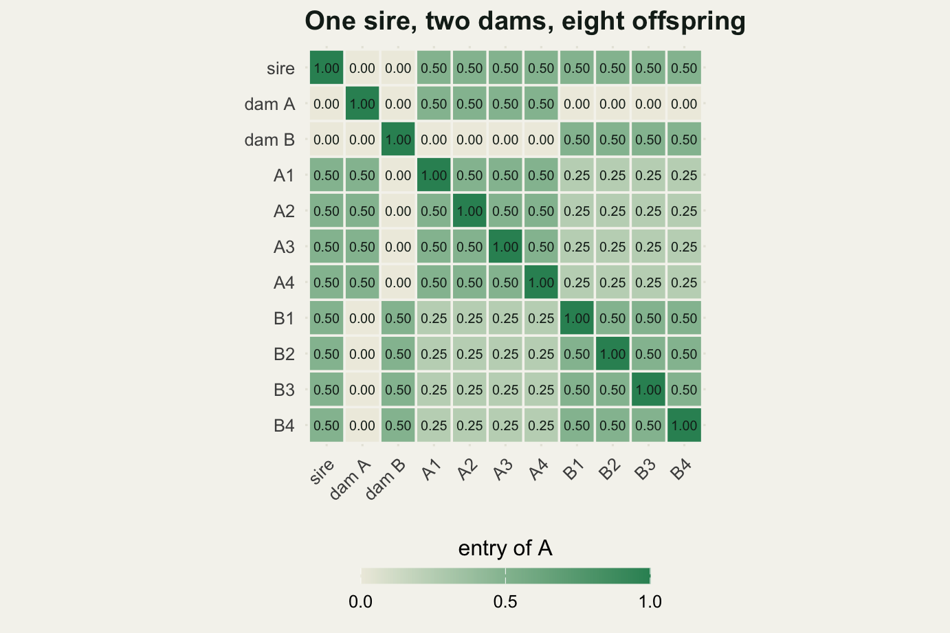
print(round(c(sire_to_A1 = sub_A[1, 4], A1_to_A2 = sub_A[4, 5],
              A1_to_B1 = sub_A[4, 8], damA_to_damB = sub_A[2, 3],
              damA_to_B1 = sub_A[2, 8]), 4))
sire_to_A1 A1_to_A2 A1_to_B1 damA_to_damB damA_to_B1
0.50 0.50 0.25 0.00 0.00 The block structure is the whole story in one picture. The sire connects to all eight offspring at 0.5, within brood A the four offspring are full sibs at 0.5, and across the two broods they are paternal half sibs at 0.25. The two dams sit at 0 with each other and at 0 with the other female’s brood, because these individuals are all in the first generation off unrelated founders. That clean picture is the special case, not the rule, which is what the table above was about.
Phenotypes, and REML written out
With \(A\) in hand the generative model is short. Each individual gets a breeding value by the standard recursion: the average of its parents’ breeding values plus a Mendelian sampling term. The Mendelian term is the deviation caused by which particular half of each parent’s genome the individual happened to receive.
The general variance of that term for an individual with two known parents is \(\tfrac{1}{2}\sigma^2_a\left(1 - \tfrac{1}{2}(F_s + F_d)\right)\), which shrinks as the parents themselves become inbred. The code uses the simplified non-inbred form: \(\sigma^2_a/2\) for two known parents, \(\tfrac{3}{4}\sigma^2_a\) for one, and \(\sigma^2_a\) for a founder. That is a real approximation and it matters here, given a mean inbreeding coefficient of 0.0267, so the chunk prints a check: the average of \(a_i^2 / A_{ii}\), which should equal \(\sigma^2_a\) if the simulated breeding values really do have covariance \(A\sigma^2_a\).
sim_bv <- function(sire, dam, sigma2_a) {
  n <- length(sire)
  bv <- numeric(n)
  for (i in seq_len(n)) {
    s <- sire[i]
    d <- dam[i]
    if (s > 0L && d > 0L) {
      bv[i] <- (bv[s] + bv[d])/2 + rnorm(1, 0, sqrt(sigma2_a/2))
    } else if (s > 0L) {
      bv[i] <- bv[s]/2 + rnorm(1, 0, sqrt(0.75*sigma2_a))
    } else if (d > 0L) {
      bv[i] <- bv[d]/2 + rnorm(1, 0, sqrt(0.75*sigma2_a))
    } else {
      bv[i] <- rnorm(1, 0, sqrt(sigma2_a))
    }
  }
  bv
}

sigma2_a_true <- 0.36
sigma2_e_true <- 0.64
bv <- sim_bv(ped$sire, ped$dam, sigma2_a_true)

is_male <- as.numeric(ped$sex == "M")
Xmat <- cbind(1, is_male)
mu_true <- 19.5
male_true <- 0.45
wing <- mu_true + male_true*is_male + bv + rnorm(n_ind, 0, sqrt(sigma2_e_true))

print(round(c(sigma2_a_true = sigma2_a_true, sigma2_e_true = sigma2_e_true,
              h2_true = sigma2_a_true/(sigma2_a_true + sigma2_e_true),
              mu_true = mu_true, male_true = male_true,
              mean_wing = mean(wing), var_wing = var(wing),
              realised_over_nominal = mean(bv^2/diag(A))/sigma2_a_true), 4))
sigma2_a_true sigma2_e_true h2_true
0.3600 0.6400 0.3600
mu_true male_true mean_wing
19.5000 0.4500 19.7317
var_wing realised_over_nominal
0.9682 0.9815 The simulated truth is \(\sigma^2_a =\) 0.36 and \(\sigma^2_e =\) 0.64, so \(h^2 =\) 0.36. The phenotype is a wing length in millimetres with a mean of 19.7317 mm and a variance of 0.9682, and males are 0.45 mm longer than females as a fixed effect. The realised check comes out at 0.9815 rather than one, so the simplified Mendelian term is a small cost at this level of inbreeding. Worth knowing, not worth fixing here.
Every individual in this simulation has a phenotype. That is not realistic (in a real study most founders are never measured) but it makes the incidence matrix \(Z\) the identity, which lets the likelihood be evaluated by an eigen-decomposition instead of a fresh matrix inverse at every step.
The model is \(y = Xb + Zu + e\) with \(u \sim N(0, A\sigma^2_a)\) and \(e \sim N(0, I\sigma^2_e)\), so the marginal covariance is \(V = ZAZ'\sigma^2_a + I\sigma^2_e\). REML maximises the restricted log-likelihood
\[\ell_R = -\tfrac{1}{2}\left(\log|V| + \log|X'V^{-1}X| + (y - X\hat{b})'V^{-1}(y - X\hat{b})\right)\]
where \(\hat{b}\) is the generalised least squares estimate at the current \(V\). The fixed effects are profiled out, so optim sees only two parameters, both on the log scale so they cannot wander negative.
With \(Z = I\) the trick is that \(V = Q\Lambda Q'\sigma^2_a + I\sigma^2_e = Q(\Lambda\sigma^2_a + I\sigma^2_e)Q'\), where \(Q\Lambda Q'\) is the eigen-decomposition of \(A\). The determinant is a sum of logs, the inverse is a division, and one decomposition up front makes every likelihood evaluation cost \(O(n^2)\) instead of \(O(n^3)\).
reml_fit <- function(y, X, G, start = c(1, 1)) {
  eg  <- eigen(G, symmetric = TRUE)
  lam <- pmax(eg$values, 0)
  Q   <- eg$vectors
  ys  <- crossprod(Q, y)
  Xs  <- crossprod(Q, X)
  neg_ll <- function(par) {
    dv <- lam*exp(par[1]) + exp(par[2])
    if (any(!is.finite(dv)) || any(dv <= 0)) return(1e12)
    XtVi  <- t(Xs/dv)
    XtViX <- XtVi %*% Xs
    ch <- chol(XtViX)
    bh <- backsolve(ch, forwardsolve(t(ch), XtVi %*% ys))
    rs <- ys - Xs %*% bh
    0.5*(sum(log(dv)) + 2*sum(log(diag(ch))) + sum(rs*rs/dv))
  }
  op <- optim(log(start), neg_ll, method = "Nelder-Mead",
              control = list(reltol = 1e-12, maxit = 2000))
  op <- optim(op$par, neg_ll, method = "Nelder-Mead",
              control = list(reltol = 1e-12, maxit = 2000))
  s2a <- exp(op$par[1])
  s2e <- exp(op$par[2])
  dv  <- lam*s2a + s2e
  XtVi <- t(Xs/dv)
  bh <- solve(XtVi %*% Xs, XtVi %*% ys)
  list(sigma2_a = s2a, sigma2_e = s2e, h2 = s2a/(s2a + s2e), coef = drop(bh),
       log_lik = -op$value, eigenvalues = lam, eigenvectors = Q, neg_ll = neg_ll)
}

fit <- reml_fit(wing, Xmat, A, start = c(0.4, 0.5))

print(round(c(sigma2_a = fit$sigma2_a, sigma2_e = fit$sigma2_e, h2 = fit$h2,
              intercept = unname(fit$coef[1]), male_effect = unname(fit$coef[2]),
              restricted_log_lik = fit$log_lik), 4))
sigma2_a sigma2_e h2 intercept
0.2955 0.6193 0.3230 19.6101
male_effect restricted_log_lik
0.4146 -164.9919 The fit returns \(\hat{\sigma}^2_a =\) 0.2955 against a true 0.36, \(\hat{\sigma}^2_e =\) 0.6193 against a true 0.64, and \(\hat{h}^2 =\) 0.323 against a true 0.36. The intercept is 19.6101 mm against 19.5 and the male effect 0.4146 mm against 0.45. The fixed effects land close; the variance components are in the right neighbourhood and no better than that, which is the honest summary of what a few hundred individuals buys you.
Nothing in reml_fit refers to pedigrees. It takes a response, a design matrix, and a symmetric positive definite matrix G. That generality is the point of the next section.
profile_a <- function(v)
  -optimize(function(le) fit$neg_ll(c(log(v), le)), c(-6, 3), tol = 1e-9)$objective
profile_e <- function(v)
  -optimize(function(la) fit$neg_ll(c(la, log(v))), c(-6, 3), tol = 1e-9)$objective

grid_a <- seq(0.02, 0.95, length.out = 45)
grid_e <- seq(0.30, 1.05, length.out = 45)
prof <- data.frame(
  component = factor(rep(c("additive genetic variance", "residual variance"), each = 45),
                     levels = c("additive genetic variance", "residual variance")),
  value = c(grid_a, grid_e),
  ll = c(vapply(grid_a, profile_a, 0), vapply(grid_e, profile_e, 0)))
marks <- data.frame(
  component = factor(rep(levels(prof$component), 2), levels = levels(prof$component)),
  x = c(fit$sigma2_a, fit$sigma2_e, sigma2_a_true, sigma2_e_true),
  what = rep(c("REML estimate", "simulated truth"), each = 2))

ggplot(prof, aes(value, ll)) +
  geom_line(colour = te_pal$forest, linewidth = 0.9) +
  geom_vline(data = marks, aes(xintercept = x, colour = what, linetype = what),
             linewidth = 0.7) +
  scale_colour_manual(values = c("REML estimate" = te_pal$green,
                                 "simulated truth" = te_pal$clay), name = NULL) +
  scale_linetype_manual(values = c("REML estimate" = "dashed",
                                   "simulated truth" = "dotted"), name = NULL) +
  facet_wrap(~component, scales = "free_x") +
  labs(x = "variance component", y = "profiled restricted log-likelihood",
       title = "Two shallow ridges") +
  theme_te()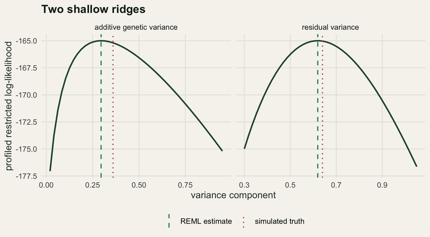
inside <- prof$ll[prof$component == "additive genetic variance"] >
          max(prof$ll[prof$component == "additive genetic variance"]) - 1.92
print(round(c(drop_used = 1.92, support_lo = min(grid_a[inside]),
              support_hi = max(grid_a[inside]),
              support_width = max(grid_a[inside]) - min(grid_a[inside])), 4))
drop_used support_lo support_hi support_width
1.9200 0.1468 0.5061 0.3593 The left panel is the one to look at. Taking the conventional 1.92 log-likelihood drop as a support interval, the additive variance is supported anywhere between 0.1468 and 0.5061 on this grid, a width of 0.3593 on a parameter whose true value is 0.36. The curve is also strongly asymmetric: it falls off a cliff towards zero and slides gently towards larger values, which is why the sampling distribution of a heritability estimate is skewed rather than symmetric and why a plus or minus standard error is a poor summary of it.
The residual variance is far better determined, which makes sense. Information about \(\sigma^2_e\) comes from the total spread of the data and there is plenty of that; information about \(\sigma^2_a\) comes only from the contrast between related and unrelated pairs, and there are far fewer effectively independent comparisons of that kind than there are birds.
The same code, handed a phylogeny
Here is the claim this post exists to make. The animal model is not a special technique belonging to quantitative genetics. It is generalised least squares with a structured covariance matrix, and the structure happens to come from a pedigree. Replace that matrix with a phylogenetic variance-covariance matrix and the same code is PGLS.
To test that rather than assert it, we need a phylogeny. The function below simulates an ultrametric tree backwards in time: with \(k\) lineages remaining it waits an exponential time with rate proportional to \(k - 1\), then merges two lineages picked at random. Under Brownian motion the covariance between two tips is the length of the path they share from the root, which is the tree height minus the age of their most recent common ancestor. Scaling by the height puts ones on the diagonal.
sim_tree_vcv <- function(n_tip) {
  clades <- as.list(seq_len(n_tip))
  split_age <- matrix(0, n_tip, n_tip)
  age <- 0
  k <- n_tip
  while (k > 1L) {
    age <- age + rexp(1, rate = k - 1)
    pick <- sample(k, 2)
    g1 <- clades[[pick[1]]]
    g2 <- clades[[pick[2]]]
    split_age[g1, g2] <- age
    split_age[g2, g1] <- age
    clades[[pick[1]]] <- c(g1, g2)
    clades[[pick[2]]] <- NULL
    k <- k - 1L
  }
  shared <- (age - split_age)/age
  diag(shared) <- 1
  shared
}

set.seed(20260704)
n_sp <- 48
Cmat <- sim_tree_vcv(n_sp)

sigma2_p_true <- 0.7
sigma2_r_true <- 0.3
log_mass <- round(rnorm(n_sp), 3)
Xsp <- cbind(1, log_mass)
range_size <- 1.2 + 0.8*log_mass +
  drop(crossprod(chol(Cmat), rnorm(n_sp)))*sqrt(sigma2_p_true) +
  rnorm(n_sp, 0, sqrt(sigma2_r_true))

print(round(c(n_species = n_sp, mean_shared = mean(Cmat[upper.tri(Cmat)]),
              max_shared = max(Cmat[upper.tri(Cmat)]),
              min_eigen = min(eigen(Cmat, symmetric = TRUE,
                                    only.values = TRUE)$values),
              sigma2_p_true = sigma2_p_true, sigma2_r_true = sigma2_r_true,
              intercept_true = 1.2, slope_true = 0.8), 4))
n_species mean_shared max_shared min_eigen sigma2_p_true
48.0000 0.2989 0.9930 0.0070 0.7000
sigma2_r_true intercept_true slope_true
0.3000 1.2000 0.8000 The tree has 48 tips. The average pair of species shares 0.2989 of the path from the root, the closest pair shares 0.993, and the smallest eigenvalue is 0.007. The simulated data are a log range size regressed on a log body mass, with a Brownian component of variance 0.7 and a species-specific residual of variance 0.3 standing in for measurement error.
Now the test. Feed this to reml_fit with Cmat where A used to be. Nothing else changes: same function, same optimiser, same profiling of the fixed effects.
fit_tree <- reml_fit(range_size, Xsp, Cmat, start = c(0.5, 0.5))

print(round(c(sigma2_phy = fit_tree$sigma2_a, sigma2_res = fit_tree$sigma2_e,
              lambda = fit_tree$h2, intercept = unname(fit_tree$coef[1]),
              slope = unname(fit_tree$coef[2]),
              restricted_log_lik = fit_tree$log_lik), 4))
sigma2_phy sigma2_res lambda intercept
0.3361 0.2671 0.5572 1.3700
slope restricted_log_lik
0.8235 -4.7621 The Brownian variance comes back as 0.3361 against a true 0.7, the residual as 0.2671 against a true 0.3, and the regression slope as 0.8235 against a true 0.8. The ratio \(\sigma^2_{phy}/(\sigma^2_{phy} + \sigma^2_{res})\) is 0.5572, which in this parameterisation is Pagel’s lambda: the animal model’s heritability and the comparative biologist’s phylogenetic signal are the same number wearing different labels. With 48 species that ratio is not well determined, and the profile below shows why.
Against that, an independent PGLS program written from scratch in a different parameterisation (total variance and lambda rather than two variance components), building \(V\) densely and inverting it with solve. If the two are the same model, the two restricted log-likelihoods must agree everywhere, not just at their optima.
pgls_log_lik <- function(sigma2_tot, lambda) {
  V  <- sigma2_tot*(lambda*Cmat + (1 - lambda)*diag(n_sp))
  Vi <- solve(V)
  XtViX <- t(Xsp) %*% Vi %*% Xsp
  bh <- solve(XtViX, t(Xsp) %*% Vi %*% range_size)
  rs <- range_size - Xsp %*% bh
  -0.5*(as.numeric(determinant(V, logarithm = TRUE)$modulus) +
        as.numeric(determinant(XtViX, logarithm = TRUE)$modulus) +
        as.numeric(t(rs) %*% Vi %*% rs))
}

check <- expand.grid(sigma2_tot = seq(0.4, 3.0, length.out = 12),
                     lambda = seq(0.05, 0.95, length.out = 12))
gap <- numeric(nrow(check))
for (i in seq_len(nrow(check))) {
  s2a <- check$sigma2_tot[i]*check$lambda[i]
  s2e <- check$sigma2_tot[i]*(1 - check$lambda[i])
  gap[i] <- abs(-fit_tree$neg_ll(log(c(s2a, s2e))) -
                pgls_log_lik(check$sigma2_tot[i], check$lambda[i]))
}

Vhat <- Cmat*fit_tree$sigma2_a + diag(n_sp)*fit_tree$sigma2_e
gls_coef <- drop(solve(t(Xsp) %*% solve(Vhat) %*% Xsp,
                       t(Xsp) %*% solve(Vhat) %*% range_size))

print(c(grid_points = nrow(check)))
grid_points
144 print(c(max_log_lik_gap = signif(max(gap), 3),
median_log_lik_gap = signif(median(gap), 3))) max_log_lik_gap median_log_lik_gap
3.55e-13 5.33e-15 print(round(c(animal_intercept = unname(fit_tree$coef[1]),
gls_intercept = unname(gls_coef[1]),
animal_slope = unname(fit_tree$coef[2]),
gls_slope = unname(gls_coef[2])), 6))animal_intercept gls_intercept animal_slope gls_slope
1.369996 1.369996 0.823482 0.823482 print(c(max_coef_gap = signif(max(abs(fit_tree$coef - gls_coef)), 3)))max_coef_gap
4.44e-16 Over 144 points spread across the parameter space, the largest disagreement between the two restricted log-likelihoods is 3.55e-13, with a median of 5.33e-15. Those are floating-point rounding, not model differences. The two programs share no code, use different parameterisations and different linear algebra, and compute the same function.
The fixed effects agree even more tightly. The single line of generalised least squares, \(\hat{b} = (X'V^{-1}X)^{-1}X'V^{-1}y\) evaluated at the fitted \(V\), gives an intercept of 1.369996 and a slope of 0.823482, against 1.369996 and 0.823482 from the animal model code, a largest difference of 4.44e-16. That is not agreement, that is identity. The animal model has been doing GLS all along; what it adds is estimating the covariance structure’s scale at the same time.
lam_grid <- seq(0.03, 0.97, length.out = 40)
prof_animal <- vapply(lam_grid, function(L)
  -optimize(function(ls) fit_tree$neg_ll(log(c(exp(ls)*L, exp(ls)*(1 - L)))),
            c(-4, 4), tol = 1e-10)$objective, 0)
prof_pgls <- vapply(lam_grid, function(L)
  -optimize(function(ls) -pgls_log_lik(exp(ls), L), c(-4, 4), tol = 1e-10)$objective, 0)
profile_gap <- max(abs(prof_animal - prof_pgls))

two <- data.frame(lambda = rep(lam_grid, 2), ll = c(prof_animal, prof_pgls),
                  code = rep(c("animal-model fitter, A replaced by C",
                               "hand-written PGLS, Pagel lambda"),
                             each = length(lam_grid)))

ggplot(two, aes(lambda, ll, colour = code, linetype = code, linewidth = code)) +
  geom_line() +
  scale_colour_manual(values = c(te_pal$sage, te_pal$clay), name = NULL) +
  scale_linetype_manual(values = c("solid", "42"), name = NULL) +
  scale_linewidth_manual(values = c(2.6, 0.9), name = NULL) +
  guides(colour = guide_legend(nrow = 2), linetype = guide_legend(nrow = 2),
         linewidth = guide_legend(nrow = 2)) +
  annotate("text", x = 0.06, y = min(two$ll) + 0.35, hjust = 0, size = 3.4,
           colour = te_pal$ink,
           label = paste("largest gap:", signif(profile_gap, 3))) +
  labs(x = "phylogenetic signal (lambda)", y = "profiled restricted log-likelihood",
       title = "Two programs, one likelihood") +
  theme_te()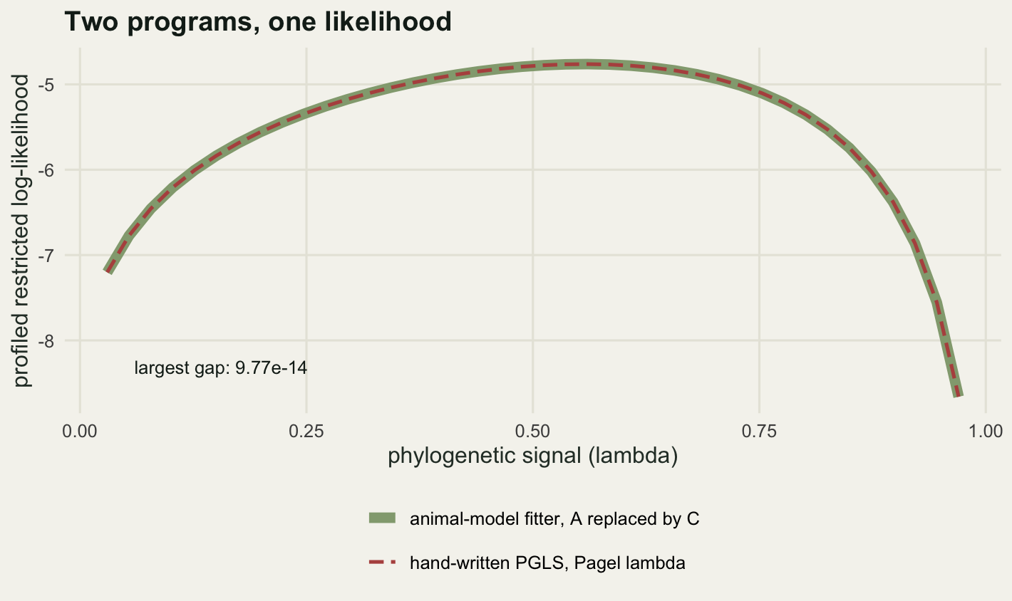
print(c(max_profile_gap = signif(profile_gap, 3)))max_profile_gap
9.77e-14 print(round(c(peak_animal = lam_grid[which.max(prof_animal)],
peak_pgls = lam_grid[which.max(prof_pgls)]), 4))peak_animal peak_pgls
0.5603 0.5603 Both curves peak at the same grid value, 0.5603, and the largest vertical gap between them anywhere along the profile is 9.77e-14. On the panel the clay dashes run down the middle of the sage band with no visible offset, which is what a gap that small looks like at plotting resolution.
The practical consequence: if you can fit an animal model you can fit PGLS, a repeatability model, a spatial model with a distance-based covariance, or a genomic relationship model, because all of them are the same likelihood with a different matrix in the same slot. What goes wrong in one goes wrong in all of them, from a badly conditioned covariance matrix to a variance component pinned against zero.
Breeding values are predictions, not measurements
Once the variance components are fixed, the breeding values follow from the mixed model equations. The BLUP of \(u\) is
\[\hat{u} = A\sigma^2_a V^{-1}(y - X\hat{b})\]
which reads as: take each individual’s deviation from the fitted mean, weight it by how much of that deviation the additive covariance can account for, and spread that information across relatives through \(A\). The prediction error variance is \(A\sigma^2_a - (A\sigma^2_a)P(A\sigma^2_a)\) with \(P\) the residual projection, and its diagonal as a proportion gives the reliability of each prediction.
dvec <- fit$eigenvalues*fit$sigma2_a + fit$sigma2_e
Vinv <- fit$eigenvectors %*% (t(fit$eigenvectors)/dvec)
resid_fixed <- wing - Xmat %*% fit$coef
u_hat <- drop(fit$sigma2_a * (A %*% (Vinv %*% resid_fixed)))

XtVi <- t(Xmat) %*% Vinv
Pmat <- Vinv - t(XtVi) %*% solve(XtVi %*% Xmat) %*% XtVi
pev  <- diag(fit$sigma2_a*A - fit$sigma2_a^2*(A %*% Pmat %*% A))
reliability <- 1 - pev/(fit$sigma2_a*diag(A))
n_close <- rowSums(A >= 0.25) - 1

slope_pred_on_true <- cov(bv, u_hat)/var(bv)
slope_true_on_pred <- cov(bv, u_hat)/var(u_hat)

print(round(c(cor_pred_true = cor(u_hat, bv), sd_predicted = sd(u_hat),
              sd_true = sd(bv), slope_pred_on_true = slope_pred_on_true,
              slope_true_on_pred = slope_true_on_pred,
              sd_ratio = sd(u_hat)/sd(bv), mean_reliability = mean(reliability),
              cor_relatives_reliability = cor(n_close, reliability)), 4))
cor_pred_true sd_predicted sd_true
0.7258 0.3912 0.6040
slope_pred_on_true slope_true_on_pred sd_ratio
0.4700 1.1206 0.6477
mean_reliability cor_relatives_reliability
0.4831 0.8415 The correlation between predicted and true breeding values is 0.7258, which is a decent result for a trait with a true heritability of 0.36 and a pedigree this shallow. The shrinkage is visible in the spread: the true breeding values have a standard deviation of 0.604 and the predictions only 0.3912.
Regressing predictions on truth gives a slope of 0.47, well below one, which is the shrinkage everyone warns about. But regressing truth on predictions gives 1.1206, close to one, and this asymmetry is the part that gets lost. A BLUP is not a shrunken guess in the sense of being systematically too small given what you know: conditional on the prediction, the expected true value is about the prediction itself. What is too small is the variance of the set of predictions, which is why feeding BLUPs to a second analysis is dangerous.
tercile <- cut(reliability, quantile(reliability, c(0, 1/3, 2/3, 1)),
               include.lowest = TRUE, labels = c("low", "middle", "high"))
idx <- seq_along(bv)
groups <- data.frame(
  reliability_group = levels(tercile),
  individuals = as.vector(table(tercile)),
  mean_close_kin = round(as.vector(tapply(n_close, tercile, mean)), 2),
  mean_reliability = round(as.vector(tapply(reliability, tercile, mean)), 4),
  slope = round(as.vector(tapply(idx, tercile,
                function(i) cov(bv[i], u_hat[i])/var(bv[i]))), 4),
  correlation = round(as.vector(tapply(idx, tercile,
                function(i) cor(bv[i], u_hat[i]))), 4),
  sd_ratio = round(as.vector(tapply(idx, tercile,
                function(i) sd(u_hat[i])/sd(bv[i]))), 4))
print(groups, row.names = FALSE)
reliability_group individuals mean_close_kin mean_reliability slope
low 130 10.40 0.3958 0.3472
middle 127 32.26 0.4907 0.4770
high 129 46.30 0.5635 0.5086
correlation sd_ratio
0.5307 0.6543
0.7691 0.6202
0.7703 0.6602Reliability tracks how many close relatives an individual has: the correlation between reliability and the count of relatives at \(A \ge 0.25\) is 0.8415. Split into terciles, the low group averages 10.4 close kin and the high group 46.3, and the regression of prediction on truth steepens from 0.3472 to 0.5086. The expected pattern holds: sparser pedigree information means heavier shrinkage.
The way it holds is not the expected way, and this is the second result worth stopping over. The ratio of predicted to true standard deviation is 0.6543 in the low group, 0.6202 in the middle and 0.6602 in the high group: essentially flat. The badly informed individuals do not get smaller predictions. They get predictions of about the same size, pointed in the wrong direction more often. The correlation is what collapses, from 0.7703 in the high group to 0.5307 in the low group, and a flatter slope with an unchanged spread is what a lower correlation looks like.
That distinction matters for anyone tempted to read a league table of predicted breeding values. An individual with two measured relatives and an extreme prediction is not being handled conservatively: its prediction is as extreme as anyone else’s and much less likely to be right.
shrink <- data.frame(true = bv, predicted = u_hat, reliability = tercile)
lines_df <- data.frame(
  slope = c(slope_pred_on_true, 1),
  intercept = c(mean(u_hat) - slope_pred_on_true*mean(bv), 0),
  kind = c("fitted shrinkage slope", "one to one"))

ggplot(shrink, aes(true, predicted, colour = reliability)) +
  geom_point(size = 1.5, alpha = 0.85) +
  geom_abline(data = lines_df, aes(slope = slope, intercept = intercept,
                                   linetype = kind),
              colour = te_pal$ink, linewidth = 0.7) +
  scale_colour_manual(values = c(low = te_pal$gold, middle = te_pal$green,
                                 high = te_pal$clay),
                      name = "reliability tercile") +
  scale_linetype_manual(values = c("fitted shrinkage slope" = "solid",
                                   "one to one" = "dashed"), name = NULL) +
  labs(x = "true breeding value (mm)", y = "predicted breeding value (mm)",
       title = "Predictions are flatter than the truth") +
  theme_te()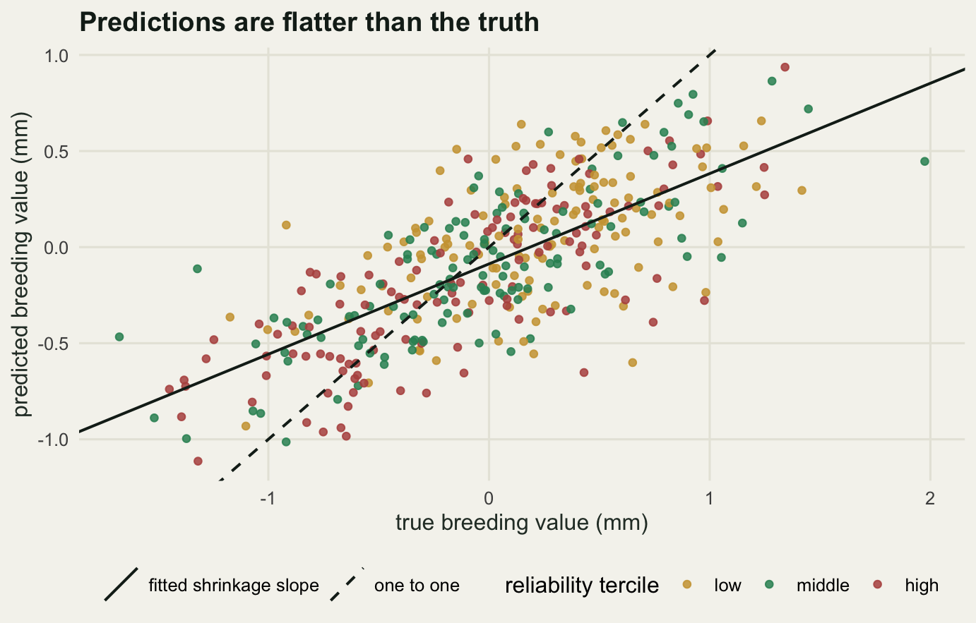
The picture is the argument. Take the predicted breeding values off the vertical axis, use them as a response in a second model (a regression of breeding value on year, say, to test for genetic change over time) and you hand that model a set of numbers whose spread is 0.6477 of the truth, whose errors are correlated with each other through the pedigree, and whose reliability varies by individual in a way the second model cannot see. Standard errors from that regression are meaningless. The fix is to put the covariate into the animal model itself, where the uncertainty in \(u\) is carried through.
What one pedigree can tell you
The fit above returned \(\hat{h}^2 =\) 0.323 when the truth was 0.36. Whether that counts as a good answer depends on how far a different pedigree of the same size would have wandered. So simulate forty fresh pedigrees of the same design, put a fresh trait on each, and fit the same model.
set.seed(20260705)
n_rep <- 40
h2_rep <- numeric(n_rep)
n_rep_ind <- numeric(n_rep)
for (r in seq_len(n_rep)) {
  pr <- sim_pedigree(80, 4, 20, 18, 4)
  Ar <- build_A(pr$sire, pr$dam)
  br <- sim_bv(pr$sire, pr$dam, sigma2_a_true)
  mr <- as.numeric(pr$sex == "M")
  yr <- mu_true + male_true*mr + br + rnorm(pr$n, 0, sqrt(sigma2_e_true))
  fr <- reml_fit(yr, cbind(1, mr), Ar, start = c(0.4, 0.5))
  h2_rep[r] <- fr$h2
  n_rep_ind[r] <- pr$n
}

print(round(c(n_replicates = n_rep, mean_pedigree_size = mean(n_rep_ind),
              h2_mean = mean(h2_rep), h2_sd = sd(h2_rep), h2_min = min(h2_rep),
              h2_max = max(h2_rep), tolerance = 0.10,
              frac_within_tolerance = mean(abs(h2_rep - 0.36) < 0.10)), 4))
n_replicates mean_pedigree_size h2_mean
40.0000 401.9750 0.3587
h2_sd h2_min h2_max
0.0896 0.2296 0.6756
tolerance frac_within_tolerance
0.1000 0.8000 Forty replicates is a small number, chosen to keep this post knitting in well under a minute, so treat the spread as indicative rather than precise. Across those 40 pedigrees, averaging 401.975 individuals each, the mean estimate is 0.3587 against a truth of 0.36, so the estimator is not badly biased. The standard deviation is 0.0896, the smallest estimate was 0.2296 and the largest 0.6756, and only 0.8 of the estimates landed within 0.10 of the truth.
Read that range again. Same generative process, same pedigree design, same number of individuals, and a single study could have reported anything from 0.2296 to 0.6756. Two studies of the same species reporting those two values are not in conflict and do not need an ecological explanation for the difference. They need more birds. Quoting a heritability to two decimal places from four hundred individuals is reporting a digit the data do not contain, and the asymmetric profile in the earlier figure says the uncertainty is not symmetric either.
What to take away
The animal model is three ideas stacked. A recursive rule that turns a parent-offspring table into a covariance matrix, a likelihood that estimates two variances given that matrix, and a linear predictor that spreads each individual’s deviation across its relatives. None of the three needs a specialist package, and writing them out makes the connections visible: the fitter that estimated additive genetic variance from a pedigree estimated Brownian variance from a phylogeny without a line changed, and agreed with an independent PGLS program to 9.77e-14 of a log-likelihood unit.
Two measured results contradict the picture most people carry. The relationship matrix does not put full sibs at 0.5: only 0.4898 of full-sib pairs were exactly 0.5, with a mean of 0.5446, because the parents are related. And shrinkage in BLUP does not work by making poorly informed predictions smaller. The predicted standard deviations were 0.6543, 0.6202 and 0.6602 of the truth across the three reliability terciles, near enough identical; what changed was the correlation, from 0.5307 to 0.7703.
The honest limit is the one the residual hides. A heritability of 0.323 is a property of this population in this environment at this time, not of wing length, and every source of resemblance the pedigree cannot resolve gets sorted into one of the two components: shared nest environment and maternal effects inflate the numerator because sibs resemble each other for reasons the model attributes to genes, while dominance and epistasis sit in the residual. Separating them needs a design that breaks the confound (cross-fostering, an extra random effect for the nest), which is what maternal effects inflate heritability measures directly. Until then, treat \(h^2\) as a description of a particular pedigree in a particular wood, and treat the interval around it as wide.
References
Henderson CR 1976 Biometrics 32(1):69-83 (10.2307/2529339)
Patterson HD, Thompson R 1971 Biometrika 58(3):545-554 (10.1093/biomet/58.3.545)
Kruuk LEB 2004 Philosophical Transactions of the Royal Society B 359(1446):873-890 (10.1098/rstb.2003.1437)
Wilson AJ, Reale D, Clements MN, Morrissey MM, Postma E, Walling CA, Kruuk LEB, Nussey DH 2010 Journal of Animal Ecology 79(1):13-26 (10.1111/j.1365-2656.2009.01639.x)
Hadfield JD, Wilson AJ, Garant D, Sheldon BC, Kruuk LEB 2010 American Naturalist 175(1):116-125 (10.1086/648604)
Freckleton RP, Harvey PH, Pagel M 2002 American Naturalist 160(6):712-726 (10.1086/343873)
Lynch M, Walsh B 1998 Genetics and Analysis of Quantitative Traits (ISBN 978-0-87893-481-2)