library(ggplot2)

te_pal <- list(forest = "#275139", green = "#2f8f63", sage = "#93a87f",
               clay = "#b5534e", gold = "#cda23f", line = "#dad9ca",
               ink = "#16241d", paper = "#f5f4ee")

theme_te <- function() {
  theme_minimal(base_size = 12) +
    theme(panel.grid.minor = element_blank(),
          panel.grid.major = element_line(colour = "#e7e6dc"),
          plot.background = element_rect(fill = "#f5f4ee", colour = NA),
          panel.background = element_rect(fill = "#f5f4ee", colour = NA),
          plot.title = element_text(face = "bold", colour = te_pal$ink),
          axis.title = element_text(colour = "#2c3a31"),
          legend.position = "bottom")
}Pedigree structure and heritability precision
R
quantitative genetics
heritability
study design
ecology tutorial
Four simulated pedigrees holding the same 480 phenotyped animals give very different heritability precision, and counting related pairs ranks them backwards.
The ringing team has been working the nest boxes for eleven springs. Every chick that fledges gets a ring, every breeding adult gets caught at the box, and the parentage is written down in a spreadsheet that now runs to several thousand rows. Somebody asks the question that always comes up over the second coffee: how many more years before we can say anything about the heritability of tarsus length?
The reflex answer is a number of birds. Five hundred, a thousand, whatever the last paper in the group’s reading list used. That answer is wrong in an interesting way, because a pedigree does not contribute information one bird at a time. It contributes information one comparison at a time, and the comparisons are between relatives. Five hundred birds with no known relatives among them carry exactly as much information about heritability as no birds at all. Not a little, not a noisy amount: none.
Between that extreme and a real study pedigree there is a lot of room, and the room is not organised the way intuition suggests. This post fixes the number of phenotyped individuals and moves only the arrangement of the relationships. Four arrangements: no relatives at all, full sib families, half sib families, and a deep pedigree running through six generations. Each one is simulated many times, the animal model is fitted to every replicate, and the spread of the heritability estimates is measured directly rather than argued about.
Two of the results are the ones everybody expects. One is not, and it is the reason the post exists: the summary of relatedness that most people reach for when they want to judge a design ranks two of these four designs in the wrong order, and by a large factor. The measurement is below, along with the summary that does get it right and the point at which that one fails too.
The machinery here, the numerator relationship matrix and the restricted likelihood that turns it into a variance component, is explained line by line in The animal model in R. This post rewrites it compactly so that it stands alone, and spends its space on the design question instead. If you want the diagnostics that tell you whether a fitted animal model can be trusted, that is Checking an animal model.
Four pedigrees, one sample size
A pedigree is three columns: an identifier, a sire and a dam, with zero standing for unknown. Everything the animal model knows about relatedness comes out of those three columns through the numerator relationship matrix \(A\), whose entry \(A_{ij}\) is twice the coefficient of kinship between individuals \(i\) and \(j\).
The matrix is built by a recursion short enough to write from memory. Process the individuals in an order that puts parents before offspring. For individual \(i\) with sire \(s\) and dam \(d\), the relationship to any earlier individual \(j\) is the average of \(j\)’s relationships to the two parents, and the diagonal is one plus half the relationship between the two parents, which is where inbreeding enters.
amat <- function(sire, dam) {
  n <- length(sire)
  A <- matrix(0, n, n)
  for (i in seq_len(n)) {
    s <- sire[i]
    d <- dam[i]
    if (i > 1L) {
      idx <- seq_len(i - 1L)
      vs <- if (s > 0L) A[idx, s] else 0
      vd <- if (d > 0L) A[idx, d] else 0
      v <- 0.5 * (vs + vd)
      A[idx, i] <- v
      A[i, idx] <- v
    }
    A[i, i] <- 1 + if (s > 0L && d > 0L) 0.5 * A[s, d] else 0
  }
  A
}

demo_sire <- c(0L, 0L, 0L, 1L, 1L, 1L, 0L, 0L, 4L, 5L)
demo_dam <- c(0L, 0L, 0L, 2L, 2L, 3L, 0L, 0L, 7L, 8L)
demo_a <- amat(demo_sire, demo_dam)
print(round(c(unrelated_founders = demo_a[1, 3],
              parent_offspring = demo_a[1, 4],
              full_sibs = demo_a[4, 5],
              half_sibs = demo_a[4, 6],
              first_cousins = demo_a[9, 10],
              diagonal = demo_a[4, 4]), 4))
unrelated_founders parent_offspring full_sibs half_sibs
0.000 0.500 0.500 0.250
first_cousins diagonal
0.125 1.000 That small pedigree is the smallest useful test of the recursion. Individuals one, two, three, seven and eight are unrelated founders; individuals four and five are full sibs from the same sire and dam; individual six shares only the sire with them; individuals nine and ten are the offspring of the two full sibs, mated to unrelated partners, which makes them first cousins. The recursion returns 0.5 between a parent and its offspring, 0.5 between full sibs, 0.25 between half sibs, 0.125 between first cousins and 0 between the unrelated founders, with 1 on the diagonal because nobody here is inbred. If that block is right, the recursion is right, and it stays right on a pedigree of a thousand rows.
Now the four designs. Each has the same number of phenotyped individuals, and in three of the four the parents exist in the pedigree but are not themselves phenotyped, which is the normal situation in a breeding experiment. The unrelated design is a set of founders with no relationships at all. The full sib design is families of four sibs each, from unrelated sire and dam pairs. The half sib design gives each sire several dams and takes one offspring per dam, so that every pair of offspring within a sire is a paternal half sib and there are no full sibs anywhere. The deep design is six generations of equal size, every generation produced by sampling sires and dams at random from the previous one, and every individual in it is phenotyped.
ped_unrelated <- function(n) {
  list(sire = rep(0L, n), dam = rep(0L, n), pheno = seq_len(n))
}

ped_fullsib <- function(nfam, ksib) {
  np <- 2L * nfam
  list(sire = c(rep(0L, np), rep(seq(1L, np, by = 2L), each = ksib)),
       dam = c(rep(0L, np), rep(seq(2L, np, by = 2L), each = ksib)),
       pheno = np + seq_len(nfam * ksib))
}

ped_halfsib <- function(nsire, ndam) {
  nd <- nsire * ndam
  np <- nsire + nd
  list(sire = c(rep(0L, np), rep(seq_len(nsire), each = ndam)),
       dam = c(rep(0L, np), nsire + seq_len(nd)),
       pheno = np + seq_len(nd))
}

ped_deep <- function(ngen, per) {
  sire <- rep(0L, per)
  dam <- rep(0L, per)
  half <- per / 2
  for (g in 2:ngen) {
    prev <- (g - 2L) * per + seq_len(per)
    sire <- c(sire, sample(prev[seq_len(half)], per, replace = TRUE))
    dam <- c(dam, sample(prev[half + seq_len(half)], per, replace = TRUE))
  }
  list(sire = sire, dam = dam, pheno = seq_len(ngen * per))
}

sub_a <- function(ped) {
  A <- amat(ped$sire, ped$dam)
  A[ped$pheno, ped$pheno]
}

n_total <- 480
n_fam <- 120
k_sib <- 4
n_sire <- 24
n_dam <- 20
n_gen <- 6
per_gen <- 80
n_rep <- 200

print(c(phenotyped = n_total, fullsib_families = n_fam, sibs_per_family = k_sib,
        pairs_per_family = choose(k_sib, 2), halfsib_sires = n_sire,
        dams_per_sire = n_dam, pairs_per_sire = choose(n_dam, 2),
        generations = n_gen, per_generation = per_gen, replicates = n_rep))
phenotyped fullsib_families sibs_per_family pairs_per_family
480 120 4 6
halfsib_sires dams_per_sire pairs_per_sire generations
24 20 190 6
per_generation replicates
80 200 set.seed(20260727)
peds <- list(unrelated = ped_unrelated(n_total),
fullsib = ped_fullsib(n_fam, k_sib),
halfsib = ped_halfsib(n_sire, n_dam),
deep = ped_deep(n_gen, per_gen))
amats <- lapply(peds, sub_a)
design_tab <- data.frame(
phenotyped = sapply(amats, nrow),
pedigree_rows = sapply(peds, function(p) length(p$sire)),
mean_diagonal = round(sapply(amats, function(A) mean(diag(A))), 4))
print(design_tab) phenotyped pedigree_rows mean_diagonal
unrelated 480 480 1.000
fullsib 480 720 1.000
halfsib 480 984 1.000
deep 480 480 1.011All four rows carry 480 phenotyped individuals, which is the point of the exercise. The pedigrees they sit in are different sizes: the unrelated design has 480 rows because the phenotyped animals are the whole pedigree, the full sib design has 720 rows once the unphenotyped parents are added, the half sib design has 984, and the deep design has 480 because everybody in it is measured.
The mean diagonal of \(A\) is 1.011 in the deep design and exactly 1 in the other three. A diagonal above one is inbreeding, and it appears in the deep design because 6 generations of random mating within 80 individuals per generation will eventually mate relatives to each other. It is a small amount of inbreeding and it drives none of the results below, but it is real and it belongs in the table.
excerpt <- list(unrelated = 1:60, fullsib = 1:60, halfsib = 1:60,
                deep = as.vector(sapply(0:5, function(g) g * per_gen + 1:10)))
design_labs <- c(unrelated = "unrelated", fullsib = "full sib",
                 halfsib = "half sib", deep = "deep")

heat_dat <- do.call(rbind, lapply(names(amats), function(nm) {
  sel <- excerpt[[nm]]
  sub <- amats[[nm]][sel, sel]
  diag(sub) <- NA_real_
  gr <- expand.grid(i = seq_along(sel), j = seq_along(sel))
  gr$r <- as.vector(sub)
  gr$design <- design_labs[[nm]]
  gr
}))
heat_dat$design <- factor(heat_dat$design, levels = design_labs)
fill_top <- max(heat_dat$r, na.rm = TRUE)

ggplot(heat_dat, aes(x = j, y = i, fill = r)) +
  geom_raster() +
  facet_wrap(~design, nrow = 1) +
  scale_y_reverse(expand = c(0, 0)) +
  scale_x_continuous(expand = c(0, 0)) +
  scale_fill_gradientn(colours = c("#e7e5d6", te_pal$sage, te_pal$green, te_pal$forest),
                       limits = c(0, fill_top), na.value = "#f5f4ee",
                       name = "relatedness") +
  coord_fixed() +
  labs(title = "The same animals, four arrangements", x = NULL, y = NULL) +
  theme_te() +
  theme(axis.text = element_blank(), panel.grid = element_blank(),
        panel.border = element_rect(colour = "#8f8d7e", fill = NA,
                                    linewidth = 0.5),
        plot.margin = margin(6, 10, 6, 10))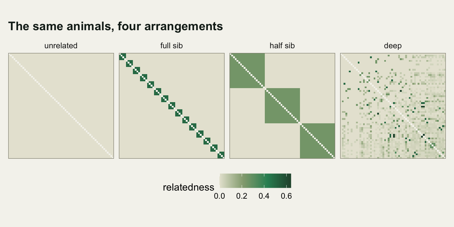
The excerpts are chosen to make each design’s block structure visible in sixty rows, so they are not the same sixty individuals in each panel: the first three panels show the first sixty phenotyped individuals, and the deep panel shows ten individuals from each of the six generations. The unrelated panel is uniform because every off-diagonal entry in it is zero. The full sib panel is a chain of small dark blocks, four by four, at 0.5. The half sib panel is three large blocks, twenty by twenty, at 0.25. The deep panel has no blocks. Its strong links are scattered singletons, a parent sitting beside its offspring wherever the two happen to fall in the ordering, and behind them a faint wash that thickens towards the later generations as everybody becomes slightly related to everybody. The top left corner, where the founders sit, is empty.
Look at the full sib and half sib panels together, because that comparison is the one the rest of the post turns on. The full sib panel has darker but much smaller blocks. The half sib panel is paler and covers far more of the square. Which of those two pictures contains more information about heritability is not obvious from looking at them, and that is exactly the question.
link_summary <- function(A) {
  off <- A[upper.tri(A)]
  ro <- round(off, 6)
  c(from_half = sum(ro >= 0.5 - 1e-6),
    from_quarter = sum(ro >= 0.25 - 1e-6 & ro < 0.5 - 1e-6),
    from_eighth = sum(ro >= 0.125 - 1e-6 & ro < 0.25 - 1e-6),
    weaker = sum(ro > 1e-6 & ro < 0.125 - 1e-6),
    any_link = sum(ro > 1e-6),
    strongest = max(off),
    sum_sq = sum(off^2))
}

link_tab <- as.data.frame(t(sapply(amats, link_summary)))
link_tab$strongest <- round(link_tab$strongest, 4)
link_tab$sum_sq <- round(link_tab$sum_sq, 2)
print(link_tab)
from_half from_quarter from_eighth weaker any_link strongest sum_sq
unrelated 0 0 0 0 0 0.00 0.00
fullsib 720 0 0 0 720 0.50 180.00
halfsib 0 4560 0 0 4560 0.25 285.00
deep 837 2180 4613 41794 49424 0.75 547.01print(c(total_pairs = choose(n_total, 2)))total_pairs
114960 There are 114960 pairs of individuals in each design. The unrelated design uses none of them: 0 pairs have a non-zero relationship. The full sib design has 720 pairs at 0.5, which is 6 pairs inside each of the 120 families, and nothing else. The half sib design has 4560 pairs at 0.25, which is 190 pairs inside each of the 24 sire groups, and nothing else. The deep design is graded rather than blocked: 837 pairs at 0.5 or stronger, the strongest of them 0.75 because some parents are themselves related, 2180 pairs between 0.25 and 0.5, 4613 between 0.125 and 0.25, and 41794 weaker than a first cousin pair, for 49424 related pairs in total.
The last column is the summary that most people reach for, and it is the one this post is going to break. Add up the squares of all the off-diagonal entries of \(A\). The squaring is not arbitrary: a squared relatedness is what appears in the Fisher information for a variance ratio, so the sum of squared relatedness looks like the right currency for judging a design. It gives 0 for the unrelated design, 180 for full sibs, 285 for half sibs and 547.01 for the deep pedigree.
On that summary the half sib design should beat the full sib design, because 285 is larger than 180. The reasoning is the one people give out loud: full sibs are related twice as strongly, but there are 6.33 times as many half sib pairs. The count wins despite the squaring, not because of it: squaring weights each full sib pair 4 times a half sib pair, and the count only just clears that, leaving half sibs ahead by a factor of 1.58. Hold that prediction. We are about to measure it.
The animal model in a few lines
The model is the standard one. Each individual has a phenotype made of a breeding value and a residual, \(y = \mu + a + e\), with \(a \sim N(0, A\sigma_a^2)\) and \(e \sim N(0, I\sigma_e^2)\). Heritability is \(h^2 = \sigma_a^2 / (\sigma_a^2 + \sigma_e^2)\). Fitting means finding the variance components that make the observed phenotypes most likely once the fixed effects have been projected out, which is what restricted maximum likelihood does.
The trick that makes hundreds of replicates cheap is to write the phenotypic covariance as \(V = \sigma_p^2 H\) with \(H = h^2 A + (1 - h^2) I\), and then to diagonalise \(A\) once per design. If \(A = U D U'\) then \(H = U (h^2 D + (1 - h^2) I) U'\), so every determinant and every solve becomes an operation on a vector of eigenvalues. Rotating the data by \(U'\) turns the fit into arithmetic on a few hundred numbers, and the total variance drops out of the restricted likelihood in closed form, leaving a one dimensional search over \(h^2\).
reml_prep <- function(A) {
  eg <- eigen(A, symmetric = TRUE)
  n <- nrow(A)
  list(d = pmax(eg$values, 1e-9), n = n,
       xt = as.numeric(crossprod(eg$vectors, rep(1, n))))
}

dev_h2 <- function(h2, st, yt) {
  lam <- h2 * st$d + (1 - h2)
  w <- 1 / lam
  xhx <- sum(st$xt^2 * w)
  xhy <- sum(st$xt * yt * w)
  yhy <- sum(yt^2 * w)
  ypy <- yhy - xhy^2 / xhx
  nm <- st$n - 1
  nm * log(ypy / nm) + sum(log(lam)) + log(xhx) + nm
}

h2_grid <- seq(0, 0.999, length.out = 61)

fit_h2 <- function(st, yt) {
  dv <- vapply(h2_grid, dev_h2, 0, st = st, yt = yt)
  k <- which.min(dv)
  lo <- h2_grid[max(1L, k - 1L)]
  hi <- h2_grid[min(length(h2_grid), k + 1L)]
  op <- optimize(dev_h2, c(lo, hi), st = st, yt = yt, tol = 1e-7)
  if (op$objective < dv[k]) op$minimum else h2_grid[k]
}

preps <- lapply(amats, reml_prep)
eig_tab <- data.frame(
  smallest = round(sapply(preps, function(s) min(s$d)), 4),
  largest = round(sapply(preps, function(s) max(s$d)), 4),
  below_one = sapply(preps, function(s) sum(s$d < 0.9999)),
  above_one = sapply(preps, function(s) sum(s$d > 1.0001)))
print(eig_tab)
smallest largest below_one above_one
unrelated 1.0000 1.0000 0 0
fullsib 0.5000 2.5000 360 120
halfsib 0.7500 5.7500 456 24
deep 0.1073 16.0507 340 125The eigenvalues are worth a moment, because they are the whole story in disguise. In the unrelated design every eigenvalue is exactly 1, since \(A\) is the identity matrix. In the full sib design there are 120 eigenvalues at 2.5, one per family, and the remaining 360 sit at 0.5. In the half sib design there are 24 large eigenvalues at 5.75, one per sire, and 456 at 0.75. The deep design has a continuous spectrum from 0.1073 to 16.0507, with 125 eigenvalues above one and 340 below it.
Each eigenvector is a contrast among the phenotypes, and its eigenvalue says how much extra variance that contrast carries if heritability is high. An eigenvalue of one means the contrast is untouched by \(h^2\), so it tells you nothing. The further an eigenvalue sits from one, in either direction, the more the contrast responds. That is the sentence to keep, and it is the sentence the sum of squared relatedness gets wrong.
sim_yt <- function(st, sa2, se2) {
  rnorm(st$n, 0, sqrt(sa2 * st$d + se2))
}

va_true <- 0.4
ve_true <- 0.6
h2_true <- va_true / (va_true + ve_true)
print(round(c(va_true = va_true, ve_true = ve_true, h2_true = h2_true), 4))
va_true ve_true h2_true
0.4 0.6 0.4 set.seed(70260727)
one_fit <- round(c(fullsib = fit_h2(preps$fullsib, sim_yt(preps$fullsib, va_true, ve_true)),
halfsib = fit_h2(preps$halfsib, sim_yt(preps$halfsib, va_true, ve_true)),
deep = fit_h2(preps$deep, sim_yt(preps$deep, va_true, ve_true))), 4)
print(one_fit)fullsib halfsib deep
0.3557 0.4155 0.3978 Because \(U'y\) has a diagonal covariance, the simulation can be written directly in the rotated space: the rotated phenotype is a vector of independent normals with variances \(\sigma_a^2 d_i + \sigma_e^2\). That is exactly equivalent to drawing breeding values from \(N(0, A\sigma_a^2)\) and adding residuals, and it costs one call to rnorm per replicate instead of a matrix multiplication. The trait is centred at zero and the model still fits an intercept, which is the fixed effect that restricted likelihood corrects for.
One simulated dataset per design, with true additive variance 0.4 and residual variance 0.6 so that the true heritability is 0.4, gives 0.3557 from the full sib pedigree, 0.4155 from the half sib pedigree and 0.3978 from the deep pedigree. Three numbers, all in the right neighbourhood, all useless on their own. A single estimate cannot tell you how precise a design is. That takes replicates.
Same sample size, very different precision
Now the three informative designs, each fitted to 200 replicate datasets, with true heritability 0.4 throughout. A couple of hundred replicates measures a standard deviation to within about five per cent, which is the resolution the argument needs, and it keeps the whole post inside a few seconds of compute.
run_cell <- function(st, sa2, se2, nrep) {
  vapply(seq_len(nrep), function(i) fit_h2(st, sim_yt(st, sa2, se2)), 0)
}

set.seed(90260727)
reps <- lapply(preps[c("fullsib", "halfsib", "deep")], run_cell,
               sa2 = va_true, se2 = ve_true, nrep = n_rep)

rep_tab <- data.frame(
  mean_h2 = round(sapply(reps, mean), 4),
  bias = round(sapply(reps, mean) - h2_true, 4),
  sd_h2 = round(sapply(reps, sd), 4),
  rmse = round(sapply(reps, function(x) sqrt(mean((x - h2_true)^2))), 4),
  frac_at_zero = round(sapply(reps, function(x) mean(x < 1e-3)), 4))
print(rep_tab)
mean_h2 bias sd_h2 rmse frac_at_zero
fullsib 0.3973 -0.0027 0.0995 0.0993 0
halfsib 0.3888 -0.0112 0.1550 0.1551 0
deep 0.3990 -0.0010 0.0849 0.0847 0Every design is close to unbiased, which is what restricted maximum likelihood is for. The biases are -0.0027 for full sibs, -0.0112 for half sibs and -0.0010 for the deep pedigree, all small compared with the sampling spread, and the fraction of replicates stuck on the zero boundary is 0, 0 and 0. So the designs can be compared on spread alone.
The spreads are 0.0995 for full sibs, 0.155 for half sibs and 0.0849 for the deep pedigree. That is the measurement, and it says two things.
The first is the expected one, and it holds: the deep pedigree is the most precise of the three at the same sample size. Its standard deviation is 1.83 times smaller than the half sib design’s and 1.17 times smaller than the full sib design’s. A pedigree that spreads its relatedness across generations, with parent to offspring links, grandparent links, cousins and everything between, extracts more from the same phenotypes than any single family structure does.
The second is not what the pair count predicted, and it is the opposite of it. The full sib design is more precise than the half sib design, by a factor of 1.56. The pair counting summary predicted the reverse, and predicted it by a factor of 1.26 in the other direction. The combined discrepancy in the ratio is a factor of 1.96, which is not a rounding problem. It is the summary being wrong.
dens_dat <- do.call(rbind, lapply(names(reps), function(nm) {
  dn <- density(reps[[nm]], from = 0, to = 1, n = 512)
  data.frame(h2 = dn$x, dens = dn$y, design = design_labs[[nm]])
}))
dens_dat$design <- factor(dens_dat$design, levels = design_labs[-1])
top <- max(dens_dat$dens)

ggplot(dens_dat, aes(x = h2, y = dens, colour = design)) +
  geom_line(linewidth = 1.1) +
  annotate("segment", x = 0, xend = 0, y = 0, yend = top * 0.55,
           colour = te_pal$sage, linewidth = 2.4) +
  annotate("text", x = 0.035, y = top * 0.62, hjust = 0, size = 3.4,
           colour = te_pal$ink, label = "unrelated: every replicate here") +
  annotate("segment", x = h2_true, xend = h2_true, y = 0, yend = top,
           colour = te_pal$ink, linetype = "dashed", linewidth = 0.6) +
  annotate("text", x = 0.02, y = top * 0.99, hjust = 0, size = 3.4,
           colour = te_pal$ink, label = "dashed line: true heritability") +
  scale_colour_manual(values = c("full sib" = te_pal$clay,
                                 "half sib" = te_pal$gold,
                                 "deep" = te_pal$forest), name = NULL) +
  coord_cartesian(xlim = c(-0.02, 1), ylim = c(0, top * 1.05), expand = FALSE) +
  labs(title = "Same animals, three arrangements",
       x = "estimated heritability", y = "density") +
  theme_te() +
  theme(plot.margin = margin(6, 14, 6, 8))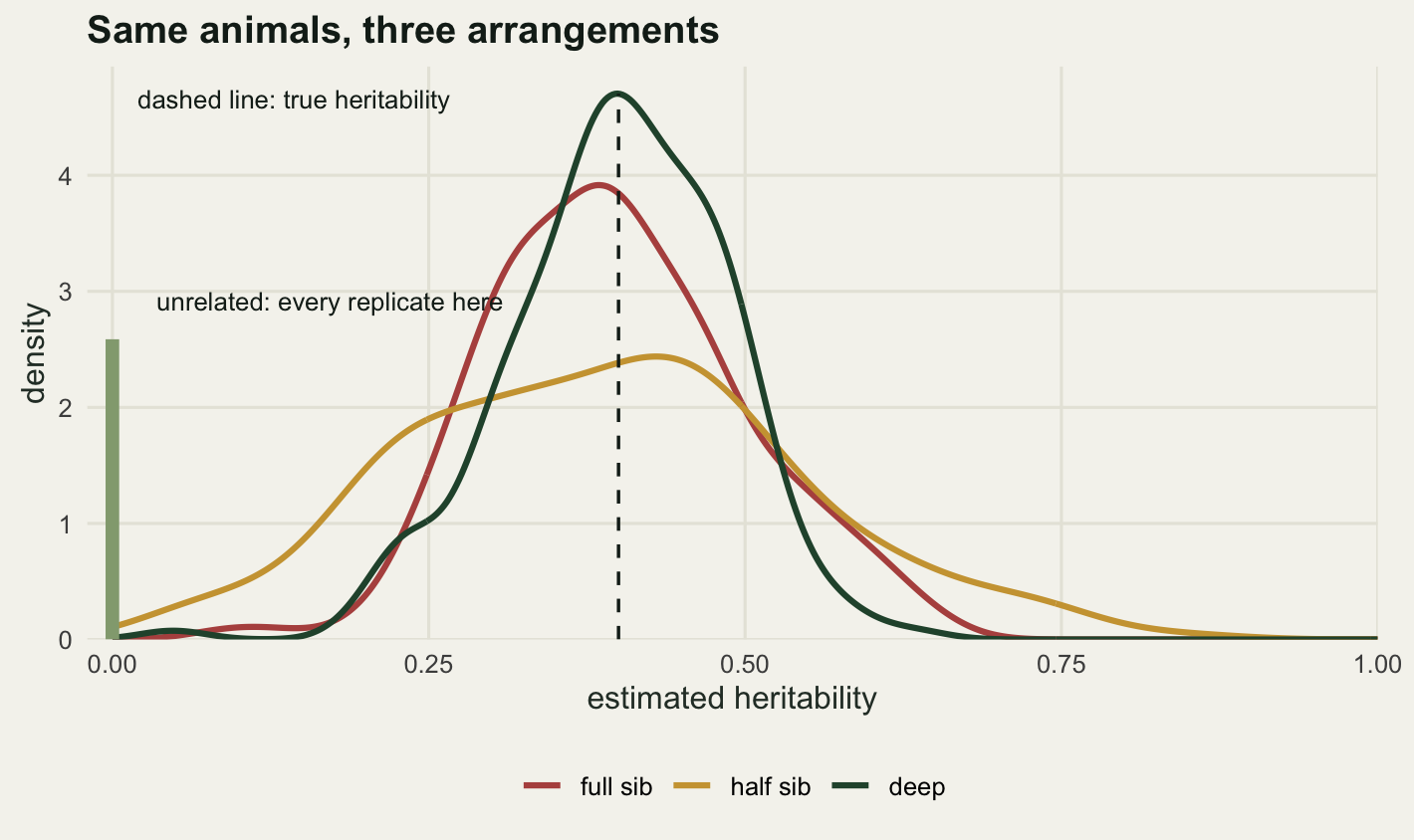
The picture makes the ordering hard to argue with. The gold half sib curve is visibly the widest of the three, and its central ninety per cent runs from 0.147 to 0.645. The red full sib curve runs from 0.254 to 0.573, and the green deep curve from 0.237 to 0.515.
Put that in the terms a reviewer will use. With the half sib design you report a heritability near 0.4 with a ninety per cent interval roughly 0.5 wide, which does not distinguish a trait with a third of its variance genetic from a trait with two thirds. With the deep design the same animals give an interval 0.28 wide. Same fieldwork, same laboratory cost, different question answered.
Sample size, and what actually predicts precision
Fix the design and vary the sample size. The half sib structure is held constant at 20 dams per sire and the number of sires is doubled three times, giving four sample sizes. If precision followed a square root rule the standard deviation would fall by a factor of \(\sqrt{2}\) at each doubling, and the slope of log standard deviation on log sample size would be exactly -0.5. That is a prediction, not a fact, so it gets measured.
n_sires <- c(3, 6, 12, 24)
size_n <- n_sires * n_dam
set.seed(60120727)
size_preps <- lapply(n_sires, function(s) reml_prep(sub_a(ped_halfsib(s, n_dam))))
names(size_preps) <- paste0("hs", size_n)
size_sumsq <- sapply(n_sires, function(s) {
  A <- sub_a(ped_halfsib(s, n_dam))
  sum(A[upper.tri(A)]^2)
})

set.seed(31415926)
size_reps <- lapply(size_preps, run_cell, sa2 = va_true, se2 = ve_true, nrep = n_rep)
size_sd <- as.numeric(sapply(size_reps, sd))
size_pred <- as.numeric(sapply(size_preps, asym_sd, h2 = h2_true))

size_tab <- data.frame(
  N = size_n,
  sum_sq = round(size_sumsq, 2),
  measured_sd = round(size_sd, 4),
  predicted_sd = round(size_pred, 4),
  bias = round(sapply(size_reps, mean) - h2_true, 4),
  rmse = round(sapply(size_reps, function(x) sqrt(mean((x - h2_true)^2))), 4),
  frac_at_zero = round(sapply(size_reps, function(x) mean(x < 1e-3)), 4))
size_tab$pred_ratio <- round(size_tab$predicted_sd / size_tab$measured_sd, 4)
print(size_tab)
N sum_sq measured_sd predicted_sd bias rmse frac_at_zero
hs60 60 35.62 0.3600 0.4373 -0.0490 0.3625 0.320
hs120 120 71.25 0.2806 0.3092 0.0133 0.2802 0.075
hs240 240 142.50 0.2141 0.2186 -0.0252 0.2150 0.015
hs480 480 285.00 0.1478 0.1546 -0.0048 0.1475 0.005
pred_ratio
hs60 1.2147
hs120 1.1019
hs240 1.0210
hs480 1.0460slope_meas <- as.numeric(coef(lm(log(size_sd) ~ log(size_n)))[2])
slope_pred <- as.numeric(coef(lm(log(size_pred) ~ log(size_n)))[2])
step_slopes <- log(size_sd[-1] / size_sd[-4]) / log(2)
slope_se <- sqrt(2) / sqrt(2 * (n_rep - 1)) / log(2)
print(round(c(measured_exponent = slope_meas), 4))measured_exponent
-0.4243 print(round(c(predicted_exponent = slope_pred), 4))predicted_exponent
-0.5 print(round(c(step_60_120 = step_slopes[1], step_120_240 = step_slopes[2],
step_240_480 = step_slopes[3], step_standard_error = slope_se), 4)) step_60_120 step_120_240 step_240_480 step_standard_error
-0.3596 -0.3902 -0.5345 0.1023 The measured exponent is -0.4243, not -0.5. The large sample calculation gives exactly -0.5, because the information is linear in the number of sires by construction, so the discrepancy is not in the design and not in the arithmetic. It is in the boundary.
At 60 offspring a fraction 0.32 of the replicates comes back exactly zero, and at 120 that fraction is 0.075. An estimator that is being squashed against a wall cannot spread out. Its standard deviation comes out smaller than the theory says, 0.36 against a predicted 0.4373 at the smallest size, and that flattering of the small samples is what makes the fitted slope shallower than -0.5.
Going from 60 to 120 the exponent is -0.3596, from 120 to 240 it is -0.3902, and from 240 to 480 it is -0.5345. Each step is a ratio of two standard deviations estimated from 200 replicates, which gives it a standard error of about 0.1023.
The small standard deviation is not a free win. The same replicates that shrink it at 60 also carry a bias of -0.049, and the floor at zero is not what puts it there: sending everything that wanted to be negative back to zero can only move the mean up, so the floor pushes the bias upwards, not down. What is left is the small sample behaviour of the estimator itself. Reporting only the standard deviation of a boundary constrained estimator makes a bad design look tidy. The root mean squared error is the honest summary at small sample size, and it is 0.3625 there against 0.1475 at 480.
curve_dat <- rbind(
  data.frame(N = size_n, value = size_sd, series = "measured, 200 replicates"),
  data.frame(N = size_n, value = size_pred, series = "large sample prediction"))

ggplot(curve_dat, aes(x = N, y = value, colour = series, linetype = series,
                      shape = series)) +
  geom_line(linewidth = 1) +
  geom_point(size = 3, stroke = 1.1) +
  scale_x_log10(breaks = size_n) +
  scale_y_log10() +
  scale_shape_manual(values = c("measured, 200 replicates" = 16,
                                "large sample prediction" = 1), name = NULL) +
  scale_colour_manual(values = c("measured, 200 replicates" = te_pal$clay,
                                 "large sample prediction" = te_pal$forest),
                      name = NULL) +
  scale_linetype_manual(values = c("measured, 200 replicates" = "solid",
                                   "large sample prediction" = "dashed"),
                        name = NULL) +
  labs(title = "Precision against sample size, half sib design",
       subtitle = paste0("fitted log log slope ", round(slope_meas, 3),
                         "; a square root rule would give -0.5"),
       x = "phenotyped offspring", y = "sd of estimated heritability") +
  theme_te() +
  theme(plot.subtitle = element_text(colour = "#2c3a31"),
        plot.margin = margin(6, 14, 6, 8))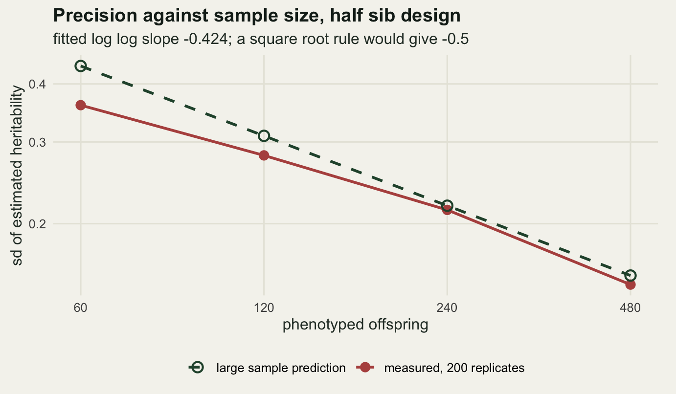
Now put the two halves together. Six distinct cells in this post have a measured standard deviation: three designs at the full sample size, and three smaller half sib designs from the size curve, whose largest point is the same design already counted. The size curve’s own estimate for that design, 0.1478, differs from the 0.155 in the main run because the two are independent sets of 200 replicates, and the gap is about what that replicate count allows. Those six span a factor of eight in sample size and a factor of 15.4 in the sum of squared relatedness. Which summary predicts the measured spread?
cells <- c("FS480", "HS480", "DEEP480", "HS60", "HS120", "HS240")
pool_sd <- c(as.numeric(sapply(reps, sd)), size_sd[1:3])
pool_sumsq <- c(link_tab$sum_sq[-1], size_sumsq[1:3])
pool_n <- c(rep(n_total, 3), size_n[1:3])
pool_pred <- c(as.numeric(sapply(preps[-1], asym_sd, h2 = h2_true)), size_pred[1:3])

pool_tab <- data.frame(cell = cells, n = pool_n,
                       sum_sq = round(pool_sumsq, 2),
                       measured_sd = round(pool_sd, 4),
                       predicted_sd = round(pool_pred, 4))
print(pool_tab)
cell n sum_sq measured_sd predicted_sd
1 FS480 480 180.00 0.0995 0.0954
2 HS480 480 285.00 0.1550 0.1546
3 DEEP480 480 547.01 0.0849 0.0780
4 HS60 60 35.62 0.3600 0.4373
5 HS120 120 71.25 0.2806 0.3092
6 HS240 240 142.50 0.2141 0.2186cor_n <- cor(log(pool_sd), log(pool_n))
cor_ss <- cor(log(pool_sd), log(pool_sumsq))
cor_pred <- cor(log(pool_sd), log(pool_pred))
print(round(c(cor_log_sd_log_n = cor_n, cor_log_sd_log_sumsq = cor_ss,
cor_log_sd_log_predicted = cor_pred), 4)) cor_log_sd_log_n cor_log_sd_log_sumsq cor_log_sd_log_predicted
-0.9176 -0.9021 0.9990 Across the six cells the correlation between log standard deviation and log sample size is -0.9176, and with the log sum of squared relatedness it is -0.9021. Those are nearly the same, and neither is a recommendation, because in this pooled set the sample size and the sum of squares move together: the size series doubles both at once. A correlation computed over a set where two candidate explanations are collinear cannot separate them, and quoting it as if it could is one of the easier ways to fool yourself.
The comparison that does separate them is the one where sample size is held fixed. At exactly 480 animals the three designs span standard deviations from 0.0849 to 0.155, a factor of 1.83, and the unrelated design at the same 480 has no precision at all. Sample size explains none of that, because sample size is constant. The sum of squared relatedness explains some of it and gets one comparison backwards. The information calculation correlates with the measured spread at 0.9990 and reproduces the values, not only the ranking.
pred_dat <- rbind(
  data.frame(cell = cells, measured = pool_sd,
             predicted = 1 / sqrt(pool_sumsq), rule = "pair counting rule"),
  data.frame(cell = cells, measured = pool_sd,
             predicted = pool_pred, rule = "REML information"))
pred_dat$rule <- factor(pred_dat$rule, levels = c("pair counting rule", "REML information"))
## the agreement line runs just above and left of the points in the right hand
## panel, so two labels are dropped below their point to keep clear of it, and
## HS120 is pushed to the right of the line instead
pred_dat$lab_vjust <- ifelse(pred_dat$cell == "DEEP480" |
                             (pred_dat$cell == "HS480" &
                              pred_dat$rule == "REML information"), 1.9, -0.9)
pred_dat$lab_hjust <- ifelse(pred_dat$cell == "HS120" &
                             pred_dat$rule == "REML information", -0.12, 0.5)

ggplot(pred_dat, aes(x = predicted, y = measured)) +
  geom_abline(slope = 1, intercept = 0, colour = te_pal$sage,
              linetype = "dashed", linewidth = 0.7) +
  geom_point(colour = te_pal$clay, size = 2.6) +
  geom_text(aes(label = cell, vjust = lab_vjust, hjust = lab_hjust),
            size = 3.1, colour = te_pal$ink) +
  facet_wrap(~rule) +
  scale_x_log10(limits = c(0.025, 0.9)) +
  scale_y_log10(limits = c(0.06, 0.6)) +
  labs(title = "Which summary predicts the measured spread",
       subtitle = "dashed line is exact agreement",
       x = "predicted sd of heritability", y = "measured sd of heritability") +
  theme_te() +
  theme(plot.subtitle = element_text(colour = "#2c3a31"),
        plot.margin = margin(6, 14, 6, 8))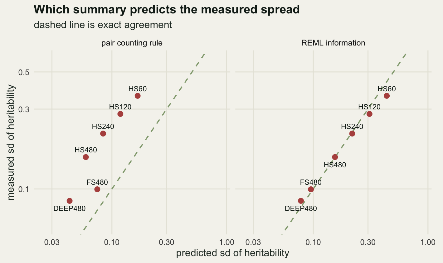
The right hand panel is what a working summary looks like: six points on the diagonal across a factor of eight in sample size and two structurally different family designs. The left hand panel is what a plausible summary looks like when it is measuring the wrong thing. It is not random, it is systematically optimistic, and it is worse than random for the one comparison that matters, because it is confident and reversed.
The practical version is four lines of R. Build \(A\) for the pedigree you are proposing, take its eigenvalues, compute \(g_i = (d_i - 1) / (h^2 d_i + 1 - h^2)\) at the heritability you expect, and the standard error of \(h^2\) is roughly \(1 / \sqrt{0.5 \sum g_i^2}\) with a small correction for the total variance. That is the asym_sd function above. It costs one eigen decomposition and it tells you, before the first animal is caught, whether the design you are about to spend three field seasons on can answer the question you are asking.
What to take away
The number of phenotyped individuals is a budget line, not a measure of information. Four pedigrees carrying the same 480 animals produced standard deviations of 0.0849, 0.0995 and 0.155, plus one design that produced no estimate at all. Arrangement did more work than sample size could have done: to match the deep design’s precision with the half sib structure you would need roughly 1600 phenotyped offspring instead of 480, and that is the optimistic figure, because it assumes the square root rate that the size curve says is not quite achieved.
The summary that survived the comparison is the restricted likelihood’s own information, computed from the eigenvalues of \(A\). The summary that failed, the sum of squared off diagonal relatedness, failed in a specific and instructive way: it is the information at zero heritability, so it ranks designs by how well they would do on a trait with no genetic variance. At a heritability of 0.4 it reversed the full sib and half sib designs, and by the same calculation the crossover between the two rankings sits at 0.08.
The honest limits are three. The first, and the one that matters most in the field: everything above measures sampling precision under a model that is correct by construction, and a design can be precise and precisely wrong. Shared environment that inflates the resemblance between sibs is measured separately in Maternal effects and shared environment, and the design this post ranks second, full sibs, is exactly the design that shared environment damages most. Precision bought by concentrating relatives into families is precision bought in the currency most vulnerable to confounding.
The second limit: the information calculation is a large sample device, and the size series shows it failing where the estimator meets the zero boundary. It over predicts the spread at 60 animals by a factor of 1.2147 and misses the bias entirely. Use it for design comparisons in the range where the estimator is not pinned, and simulate when it is. The third limit: the deep pedigree here is one random realisation with complete parentage, and real deep pedigrees have missing sires, immigrants and unequal contributions, all of which remove links and cost precision.
The habit worth keeping is small. Before the fieldwork, write down the pedigree you expect to end up with, build \(A\), and compute the standard error you will be able to report. If it comes out at 0.155 on a quantity that lives between zero and one, the study will not settle anything, and no amount of careful measurement in the field will fix a structure that has nothing to compare.
References
Wilson AJ, Reale D, Clements MN, Morrissey MB, Postma E, Walling CA, Kruuk LEB, Nussey DH 2010 Journal of Animal Ecology 79(1):13-26 (10.1111/j.1365-2656.2009.01639.x)
Kruuk LEB 2004 Philosophical Transactions of the Royal Society B 359(1446):873-890 (10.1098/rstb.2003.1437)
Kruuk LEB, Hadfield JD 2007 Journal of Evolutionary Biology 20(5):1890-1903 (10.1111/j.1420-9101.2007.01377.x)
Henderson CR 1976 Biometrics 32(1):69-83 (10.2307/2529339)
Lynch M, Walsh B 1998 Genetics and Analysis of Quantitative Traits (ISBN 978-0-87893-481-2)
Falconer DS, Mackay TFC 1996 Introduction to Quantitative Genetics, 4th edition (ISBN 978-0-582-24302-6)