library(ggplot2)
library(patchwork)

te_paper  <- "#f5f4ee"
te_ink    <- "#16241d"
te_body   <- "#2c3a31"
te_forest <- "#275139"
te_rust   <- "#b5534e"
te_gold   <- "#c9b458"
te_line   <- "#dad9ca"

theme_datasheet <- function() {
  theme_minimal(base_size = 12) +
    theme(plot.background  = element_rect(fill = te_paper, colour = NA),
          panel.background = element_rect(fill = te_paper, colour = NA),
          panel.grid.major = element_line(colour = te_line, linewidth = 0.3),
          panel.grid.minor = element_blank(),
          text             = element_text(colour = te_body),
          plot.title       = element_text(colour = te_ink, face = "bold"),
          plot.subtitle    = element_text(colour = te_body),
          axis.text        = element_text(colour = te_body),
          strip.text       = element_text(colour = te_ink, face = "bold"))
}Related founders and marker kinship in a studbook
R
conservation genetics
captive breeding
population genetics
simulation
ecology tutorial
Studbooks that treat related founders as unrelated overstate diversity; it costs breeding decisions only when sib groups differ in size. Markers tested in R.
A captive programme for a rare hamster starts from twelve animals rescued from a field colony before the plough went in. Six of them were dug out of one burrow and are a single litter. Two more burrows gave two young each, and two animals were caught alone. The studbook has no way to record any of that: a wild-caught animal gets an entry with sire and dam unknown, and every calculation downstream treats the twelve as unrelated and not inbred. The keeper then ranks animals by mean kinship, pairs them and decides how many young each pair may raise, all on a kinship matrix whose first block is wrong.
Rudnick and Lacy asked in 2008 how much that assumption costs. They simulated mean kinship programmes with 10, 30 and 100 founders, managed once on the known founder relationships and once on the assumption that the founders were unrelated, and found that knowing the relationships kept only 0 to 2 per cent more gene diversity over ten generations. The benefit was larger at higher reproductive rates and when full sibs were among a small group of founders, and they concluded that mean kinship management probably often gives near optimal results under the standard assumption. Hogg and colleagues then combined marker estimates of founder kinship with trapping records for the Tasmanian devil insurance population and found inbreeding in its first years higher than the pedigree alone had shown; replacing the assumption with a marker measurement in a real programme is their step, not this post’s. This post rebuilds the question on simulated founders whose true relationships are known and looks inside the exception Rudnick and Lacy name: whether the cost depends on how the hidden relatedness is shared out among a small group of founders, and how many markers it takes to repair it when the allele frequencies needed to read the markers have to come from the founders themselves.
Mean kinship breeding in a captive population is the direct predecessor. It compares mean kinship ranking with equal family sizes and kin avoidance, starts every run from unrelated founders, and lists related wild-caught founders among its limits as a problem it did not test. The animal model posts meet the same assumption from the other side. The animal model in R reads every founder pair at a kinship of zero and calls that an assumption, not a fact; Pedigree structure and heritability precision writes unknown parents as zeros in a three column pedigree; and the first check in Checking an animal model is about wrong sire links, not about relationships among the founders. None of them tests that assumption. For a breeding programme it is the starting point of every decision. Relatedness as a regression explains in prose why a marker estimate of relatedness depends on the population it is measured against; here that dependence turns out to decide whether a marker panel helps.
Three founder groups and what the studbook reports
The twelve founders are drawn from unrelated, non-inbred wild parents in three patterns. In the equal pattern they are four litters of three. In the unequal pattern, the hamster colony above, they are one litter of six, two litters of two and two single animals. In the half sib pattern one wild male sired six of them with six different females and the other six are unrelated. Full sibs from unrelated parents have a kinship of one quarter and half sibs one eighth; every founder has a kinship of one half with itself.
Gene diversity relative to the wild source is one minus the mean kinship over all ordered pairs of the living animals, each animal with itself included. Founder genome equivalents (FGE) are the number of unrelated, equally represented wild animals that would give the same mean kinship, one over twice the mean.
n_found <- 12
n_pop   <- 30
n_gen   <- 10
g_head  <- 6
n_rep   <- 150
n_loci  <- c(30, 100, 200, 1000)
n_ref   <- 24
founder_parents <- function(structure) {
  switch(structure,
    equal     = list(mum = rep(1:4, each = 3), dad = rep(1:4, each = 3)),
    one_large = list(mum = rep(1:5, c(6, 2, 2, 1, 1)), dad = rep(1:5, c(6, 2, 2, 1, 1))),
    half_sib  = list(mum = 1:12, dad = c(rep(1, 6), 2:7)))
}
founder_kinship <- function(parents) {
  k_f <- (outer(parents$mum, parents$mum, "==") +
          outer(parents$dad, parents$dad, "==")) / 8
  diag(k_f) <- 0.5
  k_f
}
gd_of  <- function(kin) 1 - mean(kin)
fge_of <- function(kin) 1 / (2 * mean(kin))

structures <- c("equal", "one_large", "half_sib")
k_ped <- diag(0.5, n_found)
start_tab <- t(sapply(structures, function(s) {
  k_f <- founder_kinship(founder_parents(s))
  c(gd_true = gd_of(k_f), fge_true = fge_of(k_f))
}))
gd_ped  <- gd_of(k_ped)
fge_ped <- fge_of(k_ped)
The studbook’s founder matrix is one half on the diagonal and zero elsewhere, so it reports a gene diversity of 0.958 and an FGE of 12 whatever the pattern. The true founder FGE is 6.00 for the equal litters, 4.97 for the unequal ones and 7.38 for the half sib group. That overstatement is definitional: it follows from writing zeros where the truth is a quarter or an eighth, and it needs no simulation. Whether it also changes what the keeper does is a separate question.
A marker estimate of founder kinship
Each founder is given single nucleotide polymorphism (SNP) genotypes by Mendelian transmission from its wild parents, with wild allele frequencies drawn uniformly between 0.05 and 0.5, and at most 1000 unlinked loci. Founder kinship is estimated from the genotypes as half of VanRaden’s first genomic relationship matrix: centre each allele count on twice its allele frequency, take the cross product between animals, and divide by twice the sum of the heterozygosities over loci. The diagonal is set to one half, because the founders are wild-born and assumed not inbred; a later section tests estimating it as well.
The estimator needs allele frequencies, and there are four ways to supply them. Known frequencies are the true wild values, which no real programme has. Founder frequencies are the allele frequencies among the twelve founders, which is what a programme with nothing else would use. A reference sample is 24 unrelated wild animals genotyped for the purpose. Reweighted frequencies start from the founder frequencies, estimate the kinship matrix, and then weight each founder by the row sums of the inverse of that matrix, which is the best linear unbiased estimator of McPeek and colleagues for related individuals with the true kinship replaced by its own estimate; negative estimates are set to zero for the weights, 0.01 is added to the diagonal before inversion, and the loop runs three times.
wild_genotypes <- function(parents, p_wild) {
  n_loc <- length(p_wild)
  n_mum <- max(parents$mum); n_dad <- max(parents$dad)
  hap_mum <- matrix(runif(2 * n_mum * n_loc) < rep(p_wild, each = 2 * n_mum), ncol = n_loc)
  hap_dad <- matrix(runif(2 * n_dad * n_loc) < rep(p_wild, each = 2 * n_dad), ncol = n_loc)
  geno <- matrix(0, length(parents$mum), n_loc)
  for (i in seq_along(parents$mum)) {
    from_mum <- 2 * parents$mum[i] - 1 + (runif(n_loc) < 0.5)
    from_dad <- 2 * parents$dad[i] - 1 + (runif(n_loc) < 0.5)
    geno[i, ] <- hap_mum[cbind(from_mum, seq_len(n_loc))] +
                 hap_dad[cbind(from_dad, seq_len(n_loc))]
  }
  geno
}
marker_kinship <- function(geno, p_hat, estimate_diag = FALSE) {
  keep <- p_hat > 0 & p_hat < 1
  cent <- sweep(geno[, keep, drop = FALSE], 2, 2 * p_hat[keep])
  k_hat <- tcrossprod(cent) / (2 * sum(2 * p_hat[keep] * (1 - p_hat[keep])))
  if (!estimate_diag) diag(k_hat) <- 0.5
  k_hat
}
reweighted_freq <- function(geno, n_iter = 3) {
  p_hat <- colMeans(geno) / 2
  for (it in seq_len(n_iter)) {
    k_w <- marker_kinship(geno, p_hat)
    k_w[k_w < 0] <- 0
    w_found <- solve(k_w + diag(0.01, nrow(k_w)), rep(1, nrow(k_w)))
    w_found <- w_found / sum(w_found)
    p_hat <- pmin(pmax(as.vector(crossprod(w_found, geno)) / 2, 0), 1)
  }
  p_hat
}
Managing on the wrong matrix
The breeding rule is the same for every matrix and is fixed before any run. Each generation, males and females are ranked by mean kinship; the lowest ranked male is paired with the lowest ranked female whose kinship with him is below one sixteenth, or with his least related female if none qualifies, and so on down the ranks. The census of 30 young is then handed out one at a time, each to the pair whose next offspring raises the summed kinship of the new cohort least, which may leave a pair with none. Generations are discrete, sexes are exactly balanced, and the kinship matrix of each new cohort follows from its parents by the tabular rule. The rule is run twice in parallel on the same pedigree: on the matrix the keeper believes, which makes the decisions, and on the true matrix, which scores them. A random pairing with equal family sizes (EFS) is run beside it as a reference that ignores kinship altogether.
pair_by_mk <- function(kin, male) {
  mk_rank <- rowMeans(kin)
  males <- which(male)[order(mk_rank[male])]
  fems  <- which(!male)[order(mk_rank[!male])]
  n_pair <- min(length(males), length(fems))
  pairs <- matrix(0L, n_pair, 2)
  for (k in seq_len(n_pair)) {
    below <- fems[kin[males[k], fems] < 1 / 16]
    chosen <- if (length(below)) below[1] else fems[which.min(kin[males[k], fems])]
    pairs[k, ] <- c(males[k], chosen)
    fems <- fems[fems != chosen]
  }
  pairs
}
greedy_young <- function(kin, pairs, n_off) {
  s_i <- pairs[, 1]; d_i <- pairs[, 2]
  k_between <- (kin[s_i, s_i] + kin[s_i, d_i] + kin[d_i, s_i] + kin[d_i, d_i]) / 4
  added <- (1 + kin[cbind(s_i, d_i)]) / 2
  n_young <- integer(nrow(pairs))
  for (k in seq_len(n_off)) {
    j <- which.min(added + runif(length(added), 0, 1e-9))
    n_young[j] <- n_young[j] + 1L
    added <- added + 2 * k_between[, j]
  }
  n_young
}
equal_young <- function(male, n_off) {
  males <- sample(which(male)); fems <- sample(which(!male))
  n_pair <- min(length(males), length(fems))
  n_young <- rep(n_off %/% n_pair, n_pair)
  extra <- n_off - sum(n_young)
  if (extra) { j <- sample.int(n_pair, extra); n_young[j] <- n_young[j] + 1L }
  list(pairs = cbind(males[seq_len(n_pair)], fems[seq_len(n_pair)]), n_young = n_young)
}
kin_next <- function(kin, dam, sire) {
  k_half <- (kin[dam, , drop = FALSE] + kin[sire, , drop = FALSE]) / 2
  k_off  <- (k_half[, dam, drop = FALSE] + k_half[, sire, drop = FALSE]) / 2
  diag(k_off) <- (1 + kin[cbind(dam, sire)]) / 2
  k_off
}
run_programme <- function(k_true, k_used, male_found, n_gen, rule = "mk") {
  male <- male_found
  traj <- matrix(0, n_gen, 3, dimnames = list(NULL, c("fge", "gd_rep", "f")))
  for (g in seq_len(n_gen)) {
    if (rule == "mk") {
      pairs <- pair_by_mk(k_used, male)
      n_young <- greedy_young(k_used, pairs, n_pop)
    } else {
      plan <- equal_young(male, n_pop); pairs <- plan$pairs; n_young <- plan$n_young
    }
    fam <- rep(seq_len(nrow(pairs)), n_young)
    f_new  <- k_true[cbind(pairs[fam, 1], pairs[fam, 2])]
    k_true <- kin_next(k_true, pairs[fam, 2], pairs[fam, 1])
    k_used <- kin_next(k_used, pairs[fam, 2], pairs[fam, 1])
    traj[g, ] <- c(fge_of(k_true), gd_of(k_used), mean(f_new))
    male <- sample(rep(c(TRUE, FALSE), length.out = n_pop))
  }
  traj
}
Every replicate draws one founder set, one sex assignment for the founders and one set of genotypes, and runs every matrix on those; results are compared as true FGE at generation 6 divided by the FGE that management on the true founder matrix reached from the same founders. The replication of 150 founder sets per pattern was set before the first run.
set.seed(5320)

one_founder_set <- function(structure) {
  parents <- founder_parents(structure)
  k_true  <- founder_kinship(parents)
  male_found <- sample(rep(c(TRUE, FALSE), n_found / 2))
  p_wild  <- runif(max(n_loci), 0.05, 0.5)
  geno    <- wild_genotypes(parents, p_wild)
  ref_geno <- matrix(rbinom(n_ref * max(n_loci), 2, rep(p_wild, each = n_ref)), n_ref)
  used <- list(pedigree = k_ped, oracle = k_true)
  for (n_l in n_loci) {
    g_l <- geno[, seq_len(n_l)]
    used[[paste("known", n_l)]]      <- marker_kinship(g_l, p_wild[seq_len(n_l)])
    used[[paste("founders", n_l)]]   <- marker_kinship(g_l, colMeans(g_l) / 2)
    used[[paste("reweighted", n_l)]] <- marker_kinship(g_l, reweighted_freq(g_l))
    used[[paste("reference", n_l)]]  <- marker_kinship(g_l, colMeans(ref_geno[, seq_len(n_l)]) / 2)
  }
  runs <- lapply(used, function(k_u) run_programme(k_true, k_u, male_found, n_gen))
  runs$efs <- run_programme(k_true, k_true, male_found, n_gen, rule = "efs")
  runs
}
main_sims <- lapply(setNames(structures, structures), function(s)
  replicate(n_rep, one_founder_set(s), simplify = FALSE))

arm_names <- names(main_sims[[1]][[1]])
arm_stat <- function(structure, arm, g = g_head, col = "fge") {
  v <- sapply(main_sims[[structure]], function(r) r[[arm]][g, col])
  c(mean = mean(v), se = sd(v) / sqrt(length(v)))
}
rel_to_oracle <- function(structure, arm, g = g_head) {
  d <- sapply(main_sims[[structure]], function(r)
    r[[arm]][g, "fge"] / r[["oracle"]][g, "fge"])
  c(mean = mean(d), se = sd(d) / sqrt(length(d)))
}
gd_true_of <- function(structure, arm, g = g_head) {
  mean(sapply(main_sims[[structure]], function(r) 1 - 1 / (2 * r[[arm]][g, "fge"])))
}
summ <- do.call(rbind, lapply(structures, function(s) do.call(rbind, lapply(arm_names, function(a) {
  fg <- arm_stat(s, a); rl <- rel_to_oracle(s, a)
  data.frame(structure = s, arm = a, fge = fg["mean"], fge_se = fg["se"],
             rel = rl["mean"], rel_se = rl["se"],
             gd_true = gd_true_of(s, a),
             gd_rep = arm_stat(s, a, col = "gd_rep")["mean"],
             f = arm_stat(s, a, col = "f")["mean"], row.names = NULL)
}))))
pick <- function(s, a, col = "fge") summ[summ$structure == s & summ$arm == a, col]
max_se <- max(summ$fge_se)
cost_ped <- 1 - sapply(structures, function(s) pick(s, "pedigree", "rel"))
se_ped <- sapply(structures, function(s) pick(s, "pedigree", "rel_se"))
efs_ped_gap <- max(abs(sapply(structures, function(s) pick(s, "pedigree") - pick(s, "efs"))))
gd_true_ped <- sapply(structures, function(s) pick(s, "pedigree", "gd_true"))
gd_rep_ped <- sapply(structures, function(s) pick(s, "pedigree", "gd_rep"))
f_ped <- sapply(structures, function(s) pick(s, "pedigree", "f"))
f_oracle <- sapply(structures, function(s) pick(s, "oracle", "f"))
gd_loss_large <- pick("one_large", "oracle", "gd_true") - pick("one_large", "pedigree", "gd_true")With four equal litters the pedigree matrix, which knows nothing about them, reaches 1.012 of the FGE that the true matrix reaches: nothing is lost, and the pedigree run is slightly ahead (standard error 0.0003). The benchmark is the same rule on the true matrix, not an optimum: with equal litters random pairing with equal family sizes also beats it, reaching 1.009 of it. With the litter of six the pedigree matrix reaches 0.876, a loss of 12.4 per cent of the founder genome equivalents the same rule reaches on the true matrix, and with the half sib group 0.933. On the gene diversity scale the loss for the litter of six is 0.018 (0.854 against 0.872), just under two percentage points after six generations: the upper end of what Rudnick and Lacy found, in the kind of small, sib-heavy founder group where they found a larger benefit. FGE spreads the same difference over a wider scale, which is why the post uses it for decisions. The largest Monte Carlo standard error of any mean FGE in the main grid is 0.035.
The reason shows in the EFS reference. On the pedigree matrix all twelve founders look alike, so mean kinship ranking has nothing to act on in the first generation, and the rule behaves like equal family sizes: across the three patterns the pedigree run and the EFS run differ by at most 0.013 FGE at generation 6. Equal family sizes give every founder the same share of the next generation. When the litters are equal, that also gives every wild parent pair the same share, which is what the true matrix would ask for. When one litter holds half the founders, equal shares per founder hand half of the next generation to one pair of wild genomes, and the mean kinship rule never sees it: the pedigree it works on tracks founders, not wild parent pairs.
The reported diversity is wrong in every pattern. At generation 6 the pedigree matrix reports a gene diversity of 0.909 for the unequal founders against a true 0.854, and 0.909 against 0.870 for the equal litters, where the decisions were no worse. Mean inbreeding of the generation 6 young is higher on the pedigree matrix, 0.115 against 0.086 for the unequal founders, because pairs of littermates pass the one sixteenth rule when their kinship is recorded as zero.
struct_lab <- c(equal = "four litters of three", one_large = "litter of six, 2, 2, 1, 1",
                half_sib = "six paternal half sibs")
cost_df <- summ[summ$arm %in% c("pedigree", "efs"), ]
cost_df$structure <- factor(struct_lab[cost_df$structure], levels = rev(struct_lab))
cost_df$arm <- factor(c(pedigree = "mean kinship on pedigree", efs = "equal family sizes")[cost_df$arm],
                      levels = c("mean kinship on pedigree", "equal family sizes"))
p_cost <- ggplot(cost_df, aes(rel, structure, colour = arm)) +
  geom_vline(xintercept = 1, linetype = "dashed", colour = te_body, linewidth = 0.5) +
  geom_errorbar(aes(xmin = rel - 2 * rel_se, xmax = rel + 2 * rel_se), orientation = "y",
                width = 0.2, position = position_dodge(width = 0.5)) +
  geom_point(size = 2.8, position = position_dodge(width = 0.5)) +
  scale_colour_manual(values = c(te_rust, te_gold), name = NULL) +
  labs(x = "true FGE relative to true matrix", y = NULL, title = "Decisions") +
  theme_datasheet() + theme(legend.position = "right")
rep_df <- summ[summ$arm %in% c("pedigree", "known 200", "founders 200", "reference 200"), ]
rep_df$arm <- factor(c(pedigree = "pedigree", `known 200` = "200 SNPs, known freq.",
                       `founders 200` = "200 SNPs, founder freq.",
                       `reference 200` = "200 SNPs, reference freq.")[rep_df$arm],
                     levels = c("pedigree", "200 SNPs, founder freq.", "200 SNPs, known freq.",
                                "200 SNPs, reference freq."))
rep_df$structure <- factor(struct_lab[rep_df$structure], levels = struct_lab)
p_rep <- ggplot(rep_df, aes(gd_true, gd_rep, colour = arm, shape = structure)) +
  geom_abline(slope = 1, intercept = 0, linetype = "dashed", colour = te_body, linewidth = 0.5) +
  geom_point(size = 3) +
  scale_colour_manual(values = c(te_rust, "#8c8b7c", te_forest, "#6f8fa8"), name = NULL) +
  scale_shape_manual(values = c(16, 17, 1), name = NULL) +
  scale_x_continuous(limits = c(0.845, 0.9)) +
  scale_y_continuous(limits = c(0.845, 0.96)) +
  labs(x = "true gene diversity", y = "reported gene diversity", title = "Reports") +
  theme_datasheet() + theme(legend.position = "right", legend.box = "vertical")
(p_cost / p_rep) + plot_layout(heights = c(1, 1.5)) + plot_annotation(theme = theme_datasheet())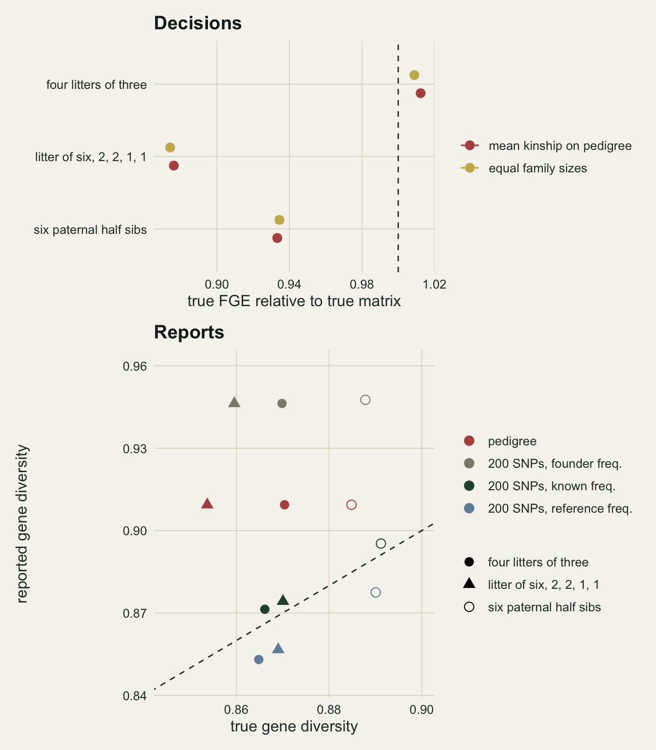
How many markers
rel_at <- function(s, src, n_l) pick(s, paste(src, n_l), "rel")
rel_se_at <- function(s, src, n_l) pick(s, paste(src, n_l), "rel_se")
known_equal <- sapply(n_loci, function(n_l) rel_at("equal", "known", n_l))
known_large <- sapply(n_loci, function(n_l) rel_at("one_large", "known", n_l))
found_large <- sapply(n_loci, function(n_l) rel_at("one_large", "founders", n_l))
reco <- function(s, src, n_l) {
  (rel_at(s, src, n_l) - pick(s, "pedigree", "rel")) / (1 - pick(s, "pedigree", "rel"))
}
With the true wild allele frequencies the marker matrix does what the pedigree cannot. For the litter of six, 30 SNPs reach 0.934 of the true matrix result, 200 SNPs 0.986 and 1000 SNPs 0.997; at 200 SNPs that is 89 per cent of the gap between the pedigree and the true matrix closed.
For the equal litters the same panels are a cost. The pedigree already matched the true matrix there, so a marker estimate can only add noise, and 30 SNPs reach 0.903 (standard error 0.004), 200 SNPs 0.980 and 1000 SNPs 0.996. A panel of a few dozen markers turns the kinship of unrelated founders from a correct zero into a scatter of positive and negative values, and the greedy allocation acts on that scatter. Founder frequencies do not share that cost here: from 100 SNPs on they give 1.006 to 1.009, level with the pedigree, for a reason the next section makes clear.
The picture changes once the frequencies come from the founders. For the litter of six, founder frequencies give 0.905 at 30 SNPs and 0.910 at 1000: more markers do not help, and at 200 SNPs they close 29 per cent of the gap. A reference sample of 24 wild animals brings the 200 SNP result back to 0.979, and the reweighted founder frequencies to 0.973. For the half sib group the founder frequencies stop at 0.957 at 1000 SNPs, against 0.998 with known frequencies.
src_lab <- c(known = "known wild frequencies", founders = "founder frequencies",
             reweighted = "reweighted founder frequencies", reference = "24 wild reference animals")
snp_df <- do.call(rbind, lapply(structures, function(s) do.call(rbind, lapply(names(src_lab), function(src)
  data.frame(structure = s, src = src, n_l = n_loci,
             rel = sapply(n_loci, function(n_l) rel_at(s, src, n_l)))))))
snp_df$src <- factor(src_lab[snp_df$src], levels = src_lab)
snp_df$structure <- factor(struct_lab[snp_df$structure], levels = struct_lab)
ped_df <- data.frame(structure = factor(struct_lab, levels = struct_lab),
                     rel = sapply(structures, function(s) pick(s, "pedigree", "rel")))
ggplot(snp_df, aes(n_l, rel, colour = src)) +
  geom_hline(yintercept = 1, colour = te_body, linewidth = 0.4) +
  geom_hline(data = ped_df, aes(yintercept = rel), linetype = "dashed", colour = te_rust,
             linewidth = 0.7) +
  geom_line(linewidth = 0.9) +
  geom_point(size = 2.2) +
  facet_wrap(~ structure, nrow = 1) +
  scale_x_log10(breaks = n_loci) +
  scale_colour_manual(values = c(te_forest, "#8c8b7c", te_gold, "#6f8fa8"), name = NULL) +
  labs(x = "SNPs (log scale)", y = "true FGE relative to true matrix") +
  theme_datasheet() + theme(legend.position = "bottom") +
  guides(colour = guide_legend(nrow = 2))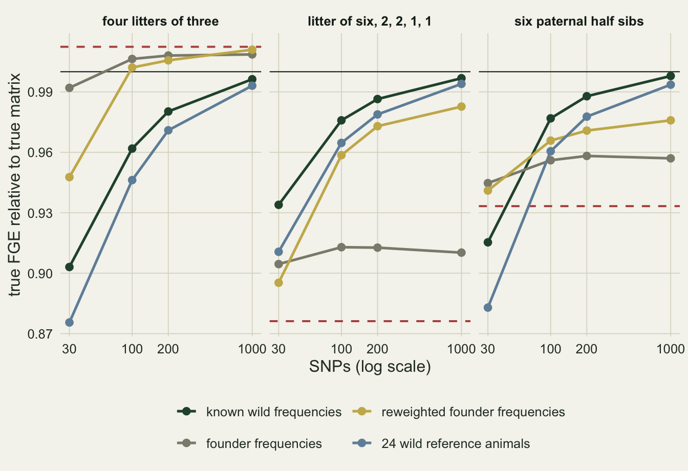
Why founder frequencies fail
set.seed(7320)
n_rep_class <- 200
class_est <- replicate(n_rep_class, {
  parents <- founder_parents("one_large"); k_true <- founder_kinship(parents)
  p_wild <- runif(200, 0.05, 0.5); geno <- wild_genotypes(parents, p_wild)
  ref_geno <- matrix(rbinom(n_ref * 200, 2, rep(p_wild, each = n_ref)), n_ref)
  big <- parents$mum == 1
  pair_class <- ifelse(outer(big, big, "&"), "within the litter of six",
                ifelse(k_true > 0, "within a pair of sibs", "unrelated"))
  up <- upper.tri(k_true)
  ests <- list(known = marker_kinship(geno, p_wild),
               founders = marker_kinship(geno, colMeans(geno) / 2),
               reweighted = marker_kinship(geno, reweighted_freq(geno)),
               reference = marker_kinship(geno, colMeans(ref_geno) / 2))
  sapply(ests, function(k_h) tapply(k_h[up], pair_class[up], mean))
}, simplify = "array")
class_mean <- apply(class_est, 1:2, mean)
p_share_big <- 6 / n_foundset.seed(9320)
n_rep_row <- 100
row_est <- replicate(n_rep_row, {
parents <- founder_parents("one_large"); k_true <- founder_kinship(parents)
p_wild <- runif(1000, 0.05, 0.5); geno <- wild_genotypes(parents, p_wild)
big <- parents$mum == 1
out <- c(row_sum = max(abs(rowSums(marker_kinship(geno, colMeans(geno) / 2, estimate_diag = TRUE)))))
for (n_l in c(200, 1000)) {
g_l <- geno[, seq_len(n_l)]
mk_f <- rowMeans(marker_kinship(g_l, colMeans(g_l) / 2))
mk_k <- rowMeans(marker_kinship(g_l, p_wild[seq_len(n_l)]))
out[paste0("gap_f", n_l)] <- mean(mk_f[big]) - mean(mk_f[!big])
out[paste0("gap_k", n_l)] <- mean(mk_k[big]) - mean(mk_k[!big])
}
out["gap_true"] <- mean(rowMeans(k_true)[big]) - mean(rowMeans(k_true)[!big])
out
})
row_gap <- rowMeans(row_est)
row_sum_max <- max(row_est["row_sum", ])A marker estimate of kinship measures how much more two animals share than two animals drawn from the reference population, and the reference is whatever the allele frequencies describe. When half of the founders are one litter, the allele frequencies among the founders are pulled half way towards that litter’s own genotypes, so its members look ordinary against a population that is half themselves. Averaged over 200 founder sets at 200 SNPs, the estimated kinship within the litter of six is 0.252 with known frequencies and 0.066 with founder frequencies, against a true value of one quarter; the littermates in the pairs of two are estimated at 0.249 and unrelated founders at -0.085. Unrelated pairs are pushed below zero, the small litters stay where they belong, and the litter of six, the one relationship the programme needed to see, is pulled down to look barely related. Centring on the founders’ own frequencies also makes every row of the estimated matrix sum to zero before the diagonal is replaced (the largest row sum over 100 founder sets at 1000 SNPs is 4.3e-15, which is rounding). Each founder’s estimated mean kinship is then one half minus its own estimated self-kinship, divided by twelve. The litter still ranks above the other founders, but the difference in mean kinship between a member of the litter of six and the other founders is 0.017 at 200 SNPs and 0.017 at 1000, against a true 0.090 and 0.091 with known frequencies. The shrinkage is a bias of the frequencies, not sampling noise, so more loci leave it where it is, and the allocation weighs a founder contrast of that size against self-kinship terms that are as large as on the true matrix. With equal litters there was no contrast to lose, as the pedigree showed.
The reweighting down-weights founders that look related, which moves the frequencies back towards the wild values and lifts the litter’s estimate to 0.116. The reference sample does not depend on the founders at all; its own sampling noise moves every estimate up a little, to 0.277 within the litter and 0.023 for unrelated pairs, which barely matters for a ranking. The zero row sums also explain the reported diversity in the bottom panel of the first figure: founder frequencies make the mean estimated kinship close to zero by construction, so the marker matrix reports a gene diversity of 0.946 at generation 6, higher than the pedigree’s own overstatement.
class_df <- do.call(rbind, lapply(dimnames(class_est)[[2]], function(src)
  data.frame(pair = rep(dimnames(class_est)[[1]], n_rep_class), src = src,
             est = as.vector(class_est[, src, ]))))
class_df$src <- factor(src_lab[class_df$src], levels = src_lab)
class_df$pair <- factor(class_df$pair, levels = c("unrelated", "within a pair of sibs",
                                                  "within the litter of six"))
ggplot(class_df, aes(src, est, fill = src)) +
  geom_hline(yintercept = c(0, 0.25), linetype = "dashed", colour = te_body, linewidth = 0.5) +
  geom_boxplot(colour = te_ink, outlier.size = 0.8, width = 0.6, linewidth = 0.4) +
  facet_wrap(~ pair, nrow = 1) +
  scale_fill_manual(values = c(te_forest, "#8c8b7c", te_gold, "#6f8fa8"), name = NULL) +
  labs(x = NULL, y = "estimated founder kinship") +
  theme_datasheet() +
  theme(axis.text.x = element_blank(), legend.position = "bottom") +
  guides(fill = guide_legend(nrow = 2))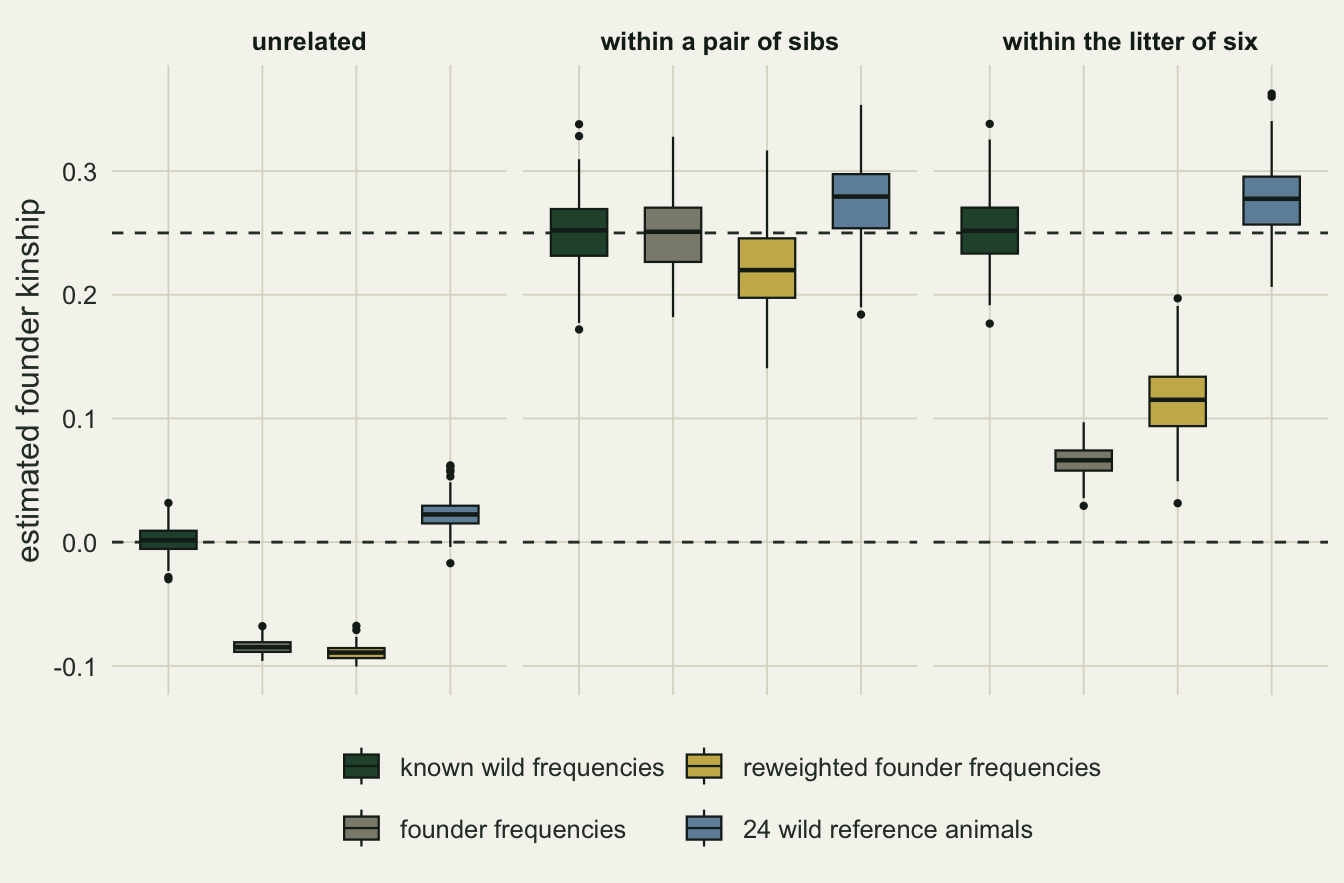
How big a litter, and for how long
set.seed(8320)
n_rep_sib <- 100
big_sizes <- c(2, 4, 6, 8, 10)
sib_parents <- function(k_big) {
  ids <- c(rep(1, k_big), 1 + seq_len(n_found - k_big))
  list(mum = ids, dad = ids)
}
sib_res <- do.call(rbind, lapply(big_sizes, function(k_big) {
  runs <- replicate(n_rep_sib, {
    parents <- sib_parents(k_big); k_true <- founder_kinship(parents)
    male_found <- sample(rep(c(TRUE, FALSE), n_found / 2))
    p_wild <- runif(200, 0.05, 0.5); geno <- wild_genotypes(parents, p_wild)
    arms <- list(oracle = k_true, pedigree = k_ped,
                 `known 200` = marker_kinship(geno, p_wild),
                 `founders 200` = marker_kinship(geno, colMeans(geno) / 2),
                 `reweighted 200` = marker_kinship(geno, reweighted_freq(geno)))
    sapply(arms, function(k_u) unname(run_programme(k_true, k_u, male_found, g_head)[g_head, "fge"]))
  })
  rel <- sweep(runs, 2, runs["oracle", ], "/")
  data.frame(k_big = k_big, arm = rownames(runs)[-1],
             rel = rowMeans(rel)[-1], se = apply(rel, 1, sd)[-1] / sqrt(n_rep_sib),
             row.names = NULL)
}))
sib_get <- function(k_big, arm) sib_res$rel[sib_res$k_big == k_big & sib_res$arm == arm]
hor_arms <- c("pedigree", "known 200", "founders 200", "reweighted 200", "reference 200")
hor_df <- do.call(rbind, lapply(hor_arms, function(a) data.frame(arm = a, gen = seq_len(n_gen),
rel = sapply(seq_len(n_gen), function(g) rel_to_oracle("one_large", a, g)["mean"]))))
hor_get <- function(a, g) hor_df$rel[hor_df$arm == a & hor_df$gen == g]The unequal pattern above mixes one large litter with two small ones. Holding everything else at single animals and varying only the size of the one litter separates the effect of its size. With a litter of two the pedigree matrix reaches 0.995 of the true matrix result; with four, 0.927; with six, 0.828; with eight, 0.757; and with ten, 0.776, from 100 founder sets each. The cost grows with the litter up to eight and stops growing at ten. A litter of six among single animals costs more than the unequal pattern of the main grid (0.828 against 0.876); the sweep does not show why the two pairs of littermates there soften the loss. Known frequencies with 200 SNPs stay between 0.985 and 0.990 over the whole range. Founder frequencies stay a few hundredths above the pedigree from a litter of four on, 0.877 at six. The reweighted frequencies repair a litter of four or six, reaching 0.974 at six, but at eight they reach 0.775 and at ten 0.809, below the founder frequencies they started from (0.813 and 0.826): when most of the founders are one litter, the first estimate is too wrong for the weights to correct it. The largest standard error in this sweep is 0.005.
Over time the cost of the pedigree matrix for the unequal founders shrinks but does not disappear within ten generations. Its share of the true matrix result is 0.814 in the first generation, 0.876 in generation 6 and 0.901 in generation 10; with founder frequencies and 200 SNPs it is 0.934 in generation 10, and with the reference sample 0.983.
arm_lab <- c(pedigree = "pedigree", `known 200` = "200 SNPs, known freq.",
             `founders 200` = "200 SNPs, founder freq.", `reweighted 200` = "200 SNPs, reweighted",
             `reference 200` = "200 SNPs, reference")
arm_cols <- setNames(c(te_rust, te_forest, "#8c8b7c", te_gold, "#6f8fa8"), arm_lab)
sib_res$arm_f <- factor(arm_lab[sib_res$arm], levels = arm_lab)
hor_df$arm_f  <- factor(arm_lab[hor_df$arm], levels = arm_lab)
p_sib <- ggplot(sib_res, aes(k_big, rel, colour = arm_f)) +
  geom_hline(yintercept = 1, colour = te_body, linewidth = 0.4) +
  geom_line(linewidth = 0.9) + geom_point(size = 2.2) +
  scale_colour_manual(values = arm_cols, limits = arm_lab, name = NULL) +
  guides(colour = guide_legend(nrow = 2)) +
  scale_x_continuous(breaks = big_sizes) +
  labs(x = "size of the one litter", y = "true FGE relative to true matrix",
       title = "Litter size") +
  theme_datasheet()
p_hor <- ggplot(hor_df, aes(gen, rel, colour = arm_f)) +
  geom_hline(yintercept = 1, colour = te_body, linewidth = 0.4) +
  geom_line(linewidth = 0.9) + geom_point(size = 2.2) +
  scale_colour_manual(values = arm_cols, limits = arm_lab, name = NULL) +
  guides(colour = guide_legend(nrow = 2)) +
  scale_x_continuous(breaks = seq(2, n_gen, 2)) +
  labs(x = "generation", y = NULL, title = "Horizon, unequal founders") +
  theme_datasheet()
(p_sib | p_hor) + plot_layout(guides = "collect") +
  plot_annotation(theme = theme_datasheet()) &
  theme(legend.position = "bottom")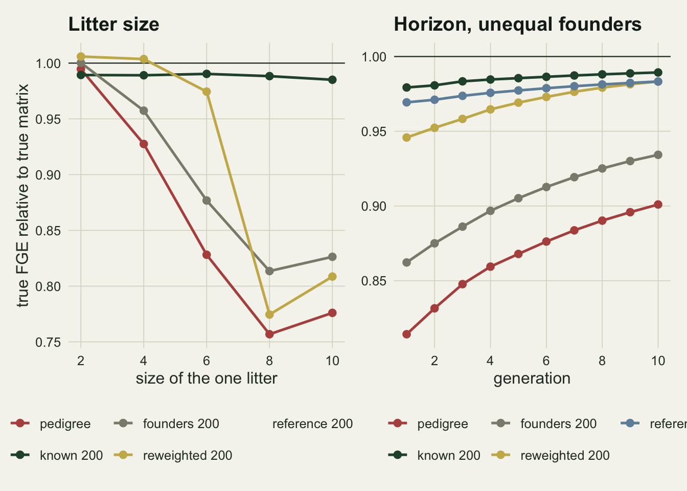
set.seed(6320)
n_rep_diag <- 150
diag_runs <- sapply(c("equal", "one_large"), function(s) rowMeans(replicate(n_rep_diag, {
  parents <- founder_parents(s); k_true <- founder_kinship(parents)
  male_found <- sample(rep(c(TRUE, FALSE), n_found / 2))
  p_wild <- runif(200, 0.05, 0.5); geno <- wild_genotypes(parents, p_wild)
  p_f <- colMeans(geno) / 2
  arms <- list(oracle = k_true,
               known_fixed = marker_kinship(geno, p_wild),
               known_est   = marker_kinship(geno, p_wild, estimate_diag = TRUE),
               found_fixed = marker_kinship(geno, p_f),
               found_est   = marker_kinship(geno, p_f, estimate_diag = TRUE))
  sapply(arms, function(k_u) unname(run_programme(k_true, k_u, male_found, g_head)[g_head, "fge"]))
})))
diag_rel <- sweep(diag_runs, 2, diag_runs["oracle", ], "/")
The founder diagonal was fixed at one half throughout. Estimating it from the markers as well, with 200 SNPs, gives 0.982 of the true matrix result for the unequal founders with known frequencies (against 0.985 with the diagonal fixed), and 0.874 with founder frequencies (against 0.911), from 150 founder sets. With the true frequencies the diagonal makes no practical difference; with founder frequencies an estimated diagonal makes a poor matrix worse. Once the diagonal is estimated too, every row of the founder frequency matrix sums to zero, so every founder’s mean kinship is zero up to rounding, the pedigree’s situation, and the result falls to about the pedigree value of 0.876 in the main grid.
What to report
Report the founder block of the kinship matrix as a choice, not as a default. A studbook analysis that states “founders assumed unrelated” should give the reported gene diversity beside that sentence, because the number is an upper bound whose distance from the truth depends on relationships nobody measured: here the pedigree reported 0.909 at generation 6 when the true value was 0.854.
Say what is known about how the founders were collected. Animals from one burrow, nest, roost or confiscated shipment are the case where the assumption misdirects breeding decisions, here by 12.4 per cent of FGE or 0.018 of gene diversity after 6 generations, a real but modest loss of the size Rudnick and Lacy reported; founders from different sites, or related in groups of the same size, are the case where it inflates the report but leaves the decisions no worse than on the true matrix.
If founder kinship comes from markers, give the number of loci and where the allele frequencies came from. With frequencies from the founders and one litter making up half of them, 1000 SNPs reached 0.910 of the true matrix result, no better than 30; a reference sample of wild animals, or a kinship-weighted estimate of the frequencies while the largest litter is not most of the founders, is part of the method, and so is the check that the estimated matrix does not report more diversity than the pedigree did.
Honest limits
Truth here is the pedigree expectation. Real founders share more or less of their genomes than their relationship predicts, and a marker estimate with many loci measures that realised sharing, which is arguably what a programme should manage; scoring the markers against the expected kinship slightly understates what a large panel is worth.
The loci are unlinked, free of genotyping error and drawn from one uniform frequency distribution, and the reference sample comes from the same wild population as the founders. Real panels have linkage, missing calls and ascertainment towards common alleles, and a reference sample from another part of the range would carry its own population structure into the founder estimates. Other relatedness estimators, including likelihood and allele sharing estimators, were not compared, and per locus standardisation of the genomic relationship matrix would weight rare alleles more heavily.
The breeding rule is one version of mean kinship management with a greedy allocation of young, the same stand-in used in the predecessor post, not the pair scores of PMx. Generations are discrete, so founders never breed again after the first round, the census is fixed and every pairing succeeds. With long-lived founders that stay in the population a keeper could correct a founder imbalance for longer, which could make a wrong founder matrix cheaper or more expensive; that was not simulated.
Markers are used only for the founders. Genotyping every generation would let the programme replace pedigree kinship altogether and would catch errors after founding too, but it costs more and is a different comparison. Founder relatedness is also only ever full sib or paternal half sib among non-inbred founders; wild populations with inbreeding or broader background relatedness among all founders would shift every founder estimate, and the half sib pattern tested is a single example.
References
Rudnick JA, Lacy RC 2008 Conservation Genetics 9(6):1439-1450 (10.1007/s10592-007-9472-2)
Hogg CJ, Wright B, Morris KM, Lee AV, Ivy JA, Grueber CE, Belov K 2019 Animal Conservation 22(4):348-361 (10.1111/acv.12463)
VanRaden PM 2008 Journal of Dairy Science 91(11):4414-4423 (10.3168/jds.2007-0980)
McPeek MS, Wu X, Ober C 2004 Biometrics 60(2):359-367 (10.1111/j.0006-341X.2004.00180.x)