library(ggplot2)
library(patchwork)

te_paper  <- "#f5f4ee"
te_ink    <- "#16241d"
te_body   <- "#2c3a31"
te_forest <- "#275139"
te_rust   <- "#b5534e"
te_gold   <- "#c9b458"
te_line   <- "#dad9ca"

theme_datasheet <- function() {
  theme_minimal(base_size = 12) +
    theme(plot.background  = element_rect(fill = te_paper, colour = NA),
          panel.background = element_rect(fill = te_paper, colour = NA),
          panel.grid.major = element_line(colour = te_line, linewidth = 0.3),
          panel.grid.minor = element_blank(),
          text             = element_text(colour = te_body),
          plot.title       = element_text(colour = te_ink, face = "bold"),
          plot.subtitle    = element_text(colour = te_body),
          axis.text        = element_text(colour = te_body))
}Mean kinship breeding in a captive population
R
conservation genetics
population genetics
captive breeding
simulation
ecology tutorial
Mean kinship breeding keeps more founder diversity than equal family sizes only when founders start unequal; unknown sires as founders undo much of it. In R.
A breeding programme for a small forest rodent starts with ten wild-caught animals, five males and five females, each pair housed on its own. In the first season one pair breeds well and produces half of the thirty young; the other four pairs share the rest. From the second season on the studbook keeper chooses who is paired with whom and how many young each pair is allowed to raise. Every choice after that first season is a genetic choice, because the population will never receive another founder, and the diversity the ten founders brought in can only be lost.
Two management rules dominate the textbooks. The older one equalises family sizes: every pair raises the same number of young, which removes the lottery in reproductive success. The one used by zoo programmes today ranks animals by mean kinship, the average kinship of an animal to everyone alive in the population including itself, and gives priority to animals whose genes are rare. Ranking by mean kinship was developed for zoo studbooks in the early 1990s and set out, together with founder genome equivalents, by Lacy in 1995; Montgomery and colleagues found in 1997 that it kept more genetic diversity than maximum avoidance of inbreeding or random breeding in replicate Drosophila populations whose founders were unequally represented, and the optimal contribution method Meuwissen published the same year, which maximises genetic gain while holding the average coancestry of the selected parents at a set value, contains the same calculation once the gain term is removed. None of that is new here. This post builds the machinery in base R, runs the rules side by side on simulated pedigrees, and measures one thing the general result does not spell out: how much mean kinship buys over equal family sizes when the founders start out evenly represented, and how much when they do not.
The site already has the pedigree algebra. The animal model in R builds the relationship matrix by the recursive rule and reads the inbreeding coefficient off its diagonal, but the matrix is there to estimate heritability, and nobody is paired on the strength of it. Effective population size in R shows that equalised family sizes nearly double Ne relative to the census, as one row of a table of formulas checked by simulation; it does not ask what a keeper who can see the pedigree should do instead. Bottlenecks and genetic diversity measures how much diversity a crash removes and ends on the point that recovery of census size is not recovery of diversity. Here the same kinship matrix is used to make the breeding decisions, and the loss it tracks is the one a closed population suffers every generation after the bottleneck of founding.
The last section turns to a problem every real studbook has: young whose sire is not known. Checking an animal model notes in passing that unknown parents point at a padding row of zeros, which is a harmless convention when the aim is a heritability estimate. In a breeding programme the zero is a statement that the animal is unrelated to everyone, and the keeper acts on it.
Kinship, gene diversity and founder genome equivalents
The kinship between two animals is the probability that a gene drawn at random from one and a gene drawn at random from the other are identical by descent. An animal’s kinship with itself is one half plus half its inbreeding coefficient, because two draws from the same animal pick the same gene copy half the time. With discrete generations the whole matrix for a new cohort follows from the matrix of its parents. Write each offspring as a row of weights on the parents, one half on its dam and one half on its sire; the kinship between two offspring is then the weighted sum of the four kinships between their parents, which is a matrix product, and the diagonal is replaced by one half plus half the kinship between each offspring’s own parents. That is the tabular method written as linear algebra, and it takes seven lines.
Two summaries of the matrix are used throughout. Mean kinship over all ordered pairs of the living cohort, the animal with itself included, is the probability that two genes drawn at random from the population are identical by descent, so gene diversity relative to the founders is one minus that mean. Founder genome equivalents, FGE, are the number of equally represented, unrelated founders that would give the same mean kinship: one over twice the mean. The two are the same number on different scales, and the definition is the whole of the connection.
next_kinship <- function(kin, dam_w, sire_w) {
  par_w   <- (dam_w + sire_w) / 2
  kin_off <- par_w %*% kin %*% t(par_w)
  f_off   <- rowSums((dam_w %*% kin) * sire_w)
  diag(kin_off) <- (1 + f_off) / 2
  list(kin = kin_off, f = f_off)
}
fge_of <- function(kin) 1 / (2 * mean(kin))

n_found   <- 10
kin_found <- diag(0.5, n_found)
fge_found <- fge_of(kin_found)
gd_found  <- 1 - mean(kin_found)

gd_target  <- 0.90
fge_target <- 1 / (2 * (1 - gd_target))
Ten unrelated, non-inbred founders have FGE 10 and a gene diversity of 0.95 on this scale; the loss from sampling ten animals out of the wild is the part that no management recovers. The target many zoo programmes quote, ninety per cent of founder gene diversity, corresponds to a mean kinship of one tenth and an FGE of 5. Both scales appear below: FGE separates the rules more visibly, gene diversity is what the programme targets are written in.
Four breeding rules, written out
The comparison is only as fair as the rules, and the mean kinship rule in particular has many versions. The four used here are fixed before any simulation runs.
Random breeding pairs males and females at random and lets family sizes fall where they fall: the thirty young are shared among the pairs by a multinomial draw with equal probabilities. Equal family size (EFS) pairs at random and gives every pair the same number of young. Kin avoidance also gives every pair the same number of young, but pairs the least related male and female first, then the least related of those left, and so on. The mean kinship rule ranks males and females by mean kinship and pairs the lowest male with the lowest female whose kinship with him is below one sixteenth, falling back to the least related female if none qualifies; it then hands out the young one at a time, each to the pair whose next offspring raises the summed kinship of the new cohort least. That greedy allocation is what gives priority to rare genes, and it is allowed to give a pair no young at all.
pair_random <- function(kin, is_male) {
  m_id <- sample(which(is_male)); f_id <- sample(which(!is_male))
  n_pair <- min(length(m_id), length(f_id))
  cbind(m_id[seq_len(n_pair)], f_id[seq_len(n_pair)])
}
pair_avoid <- function(kin, is_male) {
  m_id <- which(is_male); f_id <- which(!is_male)
  n_pair <- min(length(m_id), length(f_id))
  sub_k <- kin[m_id, f_id, drop = FALSE]
  out <- matrix(0L, n_pair, 2)
  for (k in seq_len(n_pair)) {
    hit <- which(sub_k == min(sub_k), arr.ind = TRUE)
    hit <- hit[sample.int(nrow(hit), 1), ]
    out[k, ] <- c(m_id[hit[1]], f_id[hit[2]])
    sub_k[hit[1], ] <- Inf; sub_k[, hit[2]] <- Inf
  }
  out
}
pair_mk <- function(kin, is_male) {
  mk <- rowMeans(kin) + runif(nrow(kin), 0, 1e-12)
  m_id   <- which(is_male)[order(mk[is_male])]
  f_left <- which(!is_male)[order(mk[!is_male])]
  n_pair <- min(length(m_id), length(f_left))
  out <- matrix(0L, n_pair, 2)
  for (k in seq_len(n_pair)) {
    male_k <- m_id[k]
    ok <- f_left[kin[male_k, f_left] < 1 / 16]
    fem_k <- if (length(ok)) ok[1] else f_left[which.min(kin[male_k, f_left])]
    out[k, ] <- c(male_k, fem_k); f_left <- f_left[f_left != fem_k]
  }
  out
}
alloc_equal <- function(n_pair, n_off) {
  x <- rep(n_off %/% n_pair, n_pair); r_left <- n_off - sum(x)
  if (r_left) { i <- sample.int(n_pair, r_left); x[i] <- x[i] + 1 }
  x
}
alloc_multinom <- function(n_pair, n_off) {
  as.vector(rmultinom(1, n_off, rep(1, n_pair)))
}
alloc_greedy <- function(kin, pairs, n_off) {
  s_id <- pairs[, 1]; d_id <- pairs[, 2]
  k_pp <- (kin[s_id, s_id] + kin[s_id, d_id] + kin[d_id, s_id] + kin[d_id, d_id]) / 4
  k_self <- (1 + kin[cbind(s_id, d_id)]) / 2
  cnt <- rep(0, nrow(pairs))
  for (k in seq_len(n_off)) {
    rise <- 2 * as.vector(k_pp %*% cnt) + k_self
    best <- which.min(rise + runif(length(rise), 0, 1e-9))
    cnt[best] <- cnt[best] + 1
  }
  cnt
}
The simulator keeps the census fixed, breeds one cohort per generation from the previous one, and assigns sexes to the young in exactly equal numbers. The first cohort comes from the five founder pairs with a family size vector that is part of the design: even (six young each), one prolific pair (fifteen, then four, four, four and three), or geometric (fifteen, eight, four, two, one). These sizes are for a census of thirty; at other census sizes they are scaled and rounded to whole young so that the cohort still fills the census and every founder pair keeps at least one young (at twenty: four each; ten, three, three, two, two; ten, five, three, one, one). Alongside the kinship matrix it drops two distinct alleles per founder down the same pedigree, so that the pedigree prediction can be checked against genes that were actually passed on. Generation one below is the first cohort bred from the founders.
first_cohort <- list(even      = c(6, 6, 6, 6, 6),
                     one_pair  = c(15, 4, 4, 4, 3),
                     geometric = c(15, 8, 4, 2, 1))
cohort_for <- function(skew, n_pop) {
  raw <- first_cohort[[skew]] * n_pop / 30
  x <- pmax(floor(raw), 1)
  n_left <- n_pop - sum(x)
  if (n_left > 0) {
    i <- order(raw - x, decreasing = TRUE)[seq_len(n_left)]
    x[i] <- x[i] + 1
  }
  x
}

run_line <- function(rule, skew, n_pop, n_gen) {
  kin <- kin_found
  is_male <- rep(c(TRUE, FALSE), n_found / 2)
  pairs <- cbind(which(is_male), which(!is_male))
  geno  <- matrix(seq_len(2 * n_found), n_found, 2, byrow = TRUE)
  cnt   <- cohort_for(skew, n_pop)
  out   <- matrix(0, n_gen, 7)
  for (g in seq_len(n_gen)) {
    if (g > 1) {
      pairs <- switch(rule, random = , efs = , random_greedy = pair_random(kin, is_male),
                      avoid = pair_avoid(kin, is_male),
                      mk = , mk_equal = pair_mk(kin, is_male))
      cnt <- switch(rule, random = alloc_multinom(nrow(pairs), n_pop),
                    efs = , avoid = , mk_equal = alloc_equal(nrow(pairs), n_pop),
                    mk = , random_greedy = alloc_greedy(kin, pairs, n_pop))
    }
    fam <- rep(seq_len(nrow(pairs)), cnt); n_off <- length(fam)
    dam_w  <- matrix(0, n_off, nrow(kin)); sire_w <- dam_w
    dam_w[cbind(seq_len(n_off), pairs[fam, 2])]  <- 1
    sire_w[cbind(seq_len(n_off), pairs[fam, 1])] <- 1
    step <- next_kinship(kin, dam_w, sire_w); kin <- step$kin
    geno <- cbind(geno[cbind(pairs[fam, 2], 1 + (runif(n_off) < 0.5))],
                  geno[cbind(pairs[fam, 1], 1 + (runif(n_off) < 0.5))])
    p_all <- tabulate(geno, 2 * n_found) / (2 * n_off)
    out[g, ] <- c(mean(kin), fge_of(kin), mean(step$f), 1 - sum(p_all^2),
                  sum(p_all > 0), mean(geno[, 1] != geno[, 2]),
                  if (g > 1) mean(cnt == 0) else 0)
    is_male <- sample(rep(c(TRUE, FALSE), length.out = n_off))
  }
  out
}
Even founders: equal families already do the work
The main run crosses the four rules with the three founder patterns and three census sizes, twenty, thirty and sixty, and follows each line for fifteen generations. The replication was set at 200 lines per cell before running. Everything in this section is read at a census of thirty.
n_rep  <- 200
n_gen  <- 15
rules  <- c("random", "efs", "avoid", "mk")
cells  <- expand.grid(rule = rules, skew = names(first_cohort),
                      n_pop = c(20, 30, 60), stringsAsFactors = FALSE)
set.seed(3141)
sims <- lapply(seq_len(nrow(cells)), function(i)
  replicate(n_rep, run_line(cells$rule[i], cells$skew[i], cells$n_pop[i], n_gen)))

cell_stat <- function(i, g, col) {
  v <- sims[[i]][g, col, ]
  c(mean = mean(v), se = sd(v) / sqrt(length(v)))
}
cell_id <- function(rule, skew, n_pop) {
  which(cells$rule == rule & cells$skew == skew & cells$n_pop == n_pop)
}
fge_at <- function(rule, skew, n_pop, g) cell_stat(cell_id(rule, skew, n_pop), g, 2)
f_at   <- function(rule, skew, n_pop, g) cell_stat(cell_id(rule, skew, n_pop), g, 3)

ev <- sapply(rules, function(r) fge_at(r, "even", 30, 8))
ev15 <- sapply(rules, function(r) fge_at(r, "even", 30, 15))
gap_even    <- ev["mean", "efs"] - ev["mean", "mk"]
gap_even_se <- sqrt(ev["se", "efs"]^2 + ev["se", "mk"]^2)
gap_even_pc <- 100 * gap_even / ev["mean", "efs"]
gain_rand   <- ev["mean", "efs"] / ev["mean", "random"]
gap_ea_se   <- sqrt(ev["se", "efs"]^2 + ev["se", "avoid"]^2)
After eight generations with evenly represented founders, random breeding keeps an FGE of 3.13, equal family sizes 4.40, kin avoidance 4.36 and the mean kinship rule 4.36; the largest Monte Carlo standard error among the three managed rules is 0.001. Equal family sizes keep 1.41 times the founder genome equivalents of random breeding. The three managed rules are within 1.1 per cent of each other, and the small difference that remains runs against the more elaborate rules: equal family sizes with random pairing are ahead of the mean kinship rule by 0.047 FGE, 52 standard errors. At fifteen generations the same order holds, 3.03 against 2.99.
The random breeding and EFS lines have closed form benchmarks, and they are printed here as checks of the simulator rather than as results. With a fixed census, gene diversity falls by a factor of one minus one over twice the effective size each generation. For random pairs with multinomial family sizes the variance in family size per parent is two times one minus two over the census, and the textbook approximation gives an effective size of four times the census minus two, divided by that variance plus two; with every parent raising exactly two young the variance is zero and the effective size is twice the census minus one.
n_bench  <- 30
fam_var  <- 2 * (1 - 2 / n_bench)
ne_rand  <- (4 * n_bench - 2) / (fam_var + 2)
ne_efs   <- 2 * n_bench - 1
gd_first <- 1 - cell_stat(cell_id("efs", "even", 30), 1, 1)["mean"]
gens     <- seq_len(n_gen)
gd_bench <- data.frame(gen = gens,
  random = gd_first * (1 - 1 / (2 * ne_rand))^(gens - 1),
  efs    = gd_first * (1 - 1 / (2 * ne_efs))^(gens - 1))
gd_sim_rand <- 1 - cell_stat(cell_id("random", "even", 30), n_gen, 1)["mean"]
gd_sim_efs  <- 1 - cell_stat(cell_id("efs", "even", 30), n_gen, 1)["mean"]
With a census of thirty the effective sizes are 30.5 and 59. Starting from the first cohort’s gene diversity of 0.942, the closed form gives 0.747 for random breeding at generation fifteen against a simulated 0.749, and 0.836 for equal families against 0.835.
Why kin avoidance and the mean kinship rule fall slightly behind equal families has a short algebraic answer. When every parent raises exactly two young, the pairing does not enter the mean kinship of the next cohort at all except through one term: the new mean equals the old mean plus one minus the parents’ mean inbreeding, divided by four times the census. An inbred parent’s two gene copies are already likely to be identical, so passing one of them on loses less. Pairings that keep inbreeding low therefore make the following generation lose slightly more gene diversity, not less. The chunk below checks the identity on a population taken from the simulator.
set.seed(2718)
kin_pop <- kin_found; sex_pop <- rep(c(TRUE, FALSE), 5); pr_pop <- cbind(which(sex_pop), which(!sex_pop))
for (g in 1:6) {
  if (g > 1) pr_pop <- pair_random(kin_pop, sex_pop)
  cnt_pop <- if (g > 1) alloc_equal(nrow(pr_pop), 30) else first_cohort$one_pair
  fam_pop <- rep(seq_len(nrow(pr_pop)), cnt_pop)
  dw <- matrix(0, 30, nrow(kin_pop)); sw <- dw
  dw[cbind(1:30, pr_pop[fam_pop, 2])] <- 1; sw[cbind(1:30, pr_pop[fam_pop, 1])] <- 1
  kin_pop <- next_kinship(kin_pop, dw, sw)$kin
  sex_pop <- sample(rep(c(TRUE, FALSE), 15))
}
next_mk <- function(pr) {
  fam_x <- rep(seq_len(nrow(pr)), 2)
  dw <- matrix(0, 30, 30); sw <- dw
  dw[cbind(1:30, pr[fam_x, 2])] <- 1; sw[cbind(1:30, pr[fam_x, 1])] <- 1
  mean(next_kinship(kin_pop, dw, sw)$kin)
}
f_par     <- mean(2 * diag(kin_pop) - 1)
mk_rule   <- mean(kin_pop) + (1 - f_par) / (4 * 30)
mk_random <- next_mk(pair_random(kin_pop, sex_pop))
mk_avoid  <- next_mk(pair_avoid(kin_pop, sex_pop))
id_gap    <- max(abs(c(mk_random, mk_avoid) - mk_rule))
For a population after six generations with mean inbreeding 0.1028, the formula gives a next mean kinship of 0.132616; random pairing gives 0.132616 and kin avoidance 0.132616, a largest difference of 2.78e-17, which is rounding. The generation eight FGE gap between equal families and kin avoidance, 0.048 with a standard error of 0.0009, is that inbreeding term accumulated over seven rounds of breeding. The size of the effect is a matter of the definition of gene diversity, which counts an animal’s kinship with itself; it is too small to matter to a keeper, but it means the even founder case is a tie in practice and not a win for the more elaborate rules.
traj <- do.call(rbind, lapply(which(cells$n_pop == 30 & cells$skew != "geometric"), function(i)
  data.frame(gen = gens, fge = apply(sims[[i]][, 2, ], 1, mean), rule = cells$rule[i],
             skew = cells$skew[i])))
rule_lab <- c(random = "random breeding", efs = "equal family size",
              avoid = "kin avoidance", mk = "mean kinship")
skew_lab <- c(even = "even founders", one_pair = "one pair raised half of cohort 1")
traj$rule <- factor(rule_lab[traj$rule], levels = rule_lab)
traj$skew <- factor(skew_lab[traj$skew], levels = skew_lab)
bench_long <- rbind(data.frame(gen = gens, fge = 1 / (2 * (1 - gd_bench$random)), rule = unname(rule_lab["random"])),
                    data.frame(gen = gens, fge = 1 / (2 * (1 - gd_bench$efs)), rule = unname(rule_lab["efs"])))
bench_long$rule <- factor(bench_long$rule, levels = rule_lab)
bench_long$skew <- factor(skew_lab["even"], levels = skew_lab)
rule_cols <- c(te_line, te_gold, te_rust, te_forest)
names(rule_cols) <- rule_lab
rule_cols[1] <- "#8c8b7c"

ggplot(traj, aes(gen, fge, colour = rule)) +
  geom_line(data = bench_long, linetype = "dotted", linewidth = 0.8, show.legend = FALSE) +
  geom_line(linewidth = 0.9) +
  geom_point(size = 1.4) +
  facet_wrap(~ skew) +
  scale_colour_manual(values = rule_cols, name = NULL) +
  scale_y_continuous(limits = c(0, NA)) +
  labs(x = "generation", y = "founder genome equivalents",
       title = "Mean kinship pulls ahead only from an uneven start",
       subtitle = "ten founders, census thirty; dotted: closed form benchmarks") +
  theme_datasheet() +
  theme(legend.position = "bottom", strip.text = element_text(colour = te_ink, face = "bold"))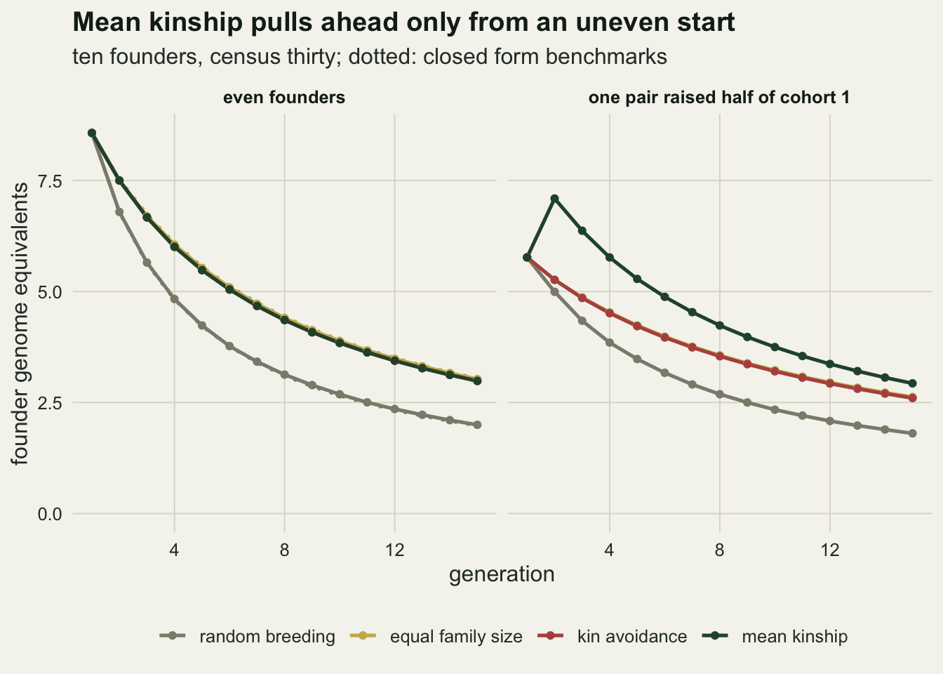
One prolific pair changes the answer
sk  <- sapply(rules, function(r) fge_at(r, "one_pair", 30, 8))
sk15 <- sapply(rules, function(r) fge_at(r, "one_pair", 30, 15))
gain8  <- 100 * (sk["mean", "mk"] / sk["mean", "efs"] - 1)
gain15 <- 100 * (sk15["mean", "mk"] / sk15["mean", "efs"] - 1)
fge_first_skew <- fge_of(next_kinship(kin_found,
  diag(1, 10)[rep(seq(2, 10, 2), first_cohort$one_pair), ],
  diag(1, 10)[rep(seq(1, 9, 2), first_cohort$one_pair), ])$kin)
fge_first_even <- fge_of(next_kinship(kin_found,
  diag(1, 10)[rep(seq(2, 10, 2), first_cohort$even), ],
  diag(1, 10)[rep(seq(1, 9, 2), first_cohort$even), ])$kin)
gd_sk <- 1 - sapply(rules, function(r) cell_stat(cell_id(r, "one_pair", 30), 8, 1)["mean"])
names(gd_sk) <- rules
zero_share <- mean(sims[[cell_id("mk", "one_pair", 30)]][2:8, 7, ])
zero_share2 <- mean(sims[[cell_id("mk", "one_pair", 30)]][2, 7, ])
fge_mk_g2   <- fge_at("mk", "one_pair", 30, 2)["mean"]
gd_gap_pts  <- 100 * (1 - cell_stat(cell_id("mk", "one_pair", 30), 8, 1)["mean"] -
                        (1 - cell_stat(cell_id("efs", "one_pair", 30), 8, 1)["mean"]))

set.seed(1618)
decomp <- sapply(c("mk_equal", "random_greedy"), function(r) {
  v <- replicate(n_rep, run_line(r, "one_pair", 30, n_gen))
  c(mean8 = mean(v[8, 2, ]), se8 = sd(v[8, 2, ]) / sqrt(n_rep), mean15 = mean(v[15, 2, ]))
})
alloc_part  <- (decomp["mean8", "random_greedy"] - sk["mean", "efs"]) / (sk["mean", "mk"] - sk["mean", "efs"])
pair_part   <- (decomp["mean8", "mk_equal"] - sk["mean", "efs"]) / (sk["mean", "mk"] - sk["mean", "efs"])
The first cohort already carries the damage. Evenly bred, it has an FGE of 8.57; with one pair raising half of it, 5.77. What the rules do afterwards now differs. At generation eight random breeding keeps 2.69, equal family sizes 3.56, kin avoidance 3.54 and the mean kinship rule 4.24: 19 per cent more than equal families, with standard errors no larger than 0.0016. Equal family sizes stop the imbalance from getting worse but copy it forward, because every pair raises the same number of young whatever share of the prolific founders it carries. The mean kinship rule reads the imbalance off the matrix and gives more young to descendants of the four under-represented pairs.
The advantage shrinks with time. By generation fifteen the figures are 2.62 for equal families and 2.93 for mean kinship, a gain of 12 per cent. Once the founder representation has been evened out, which takes the mean kinship rule a few generations, the two rules lose diversity at nearly the same rate, and the head start is a fixed amount of FGE on a shrinking total. On the gene diversity scale the generation eight difference is 0.882 against 0.860, which sounds small and is the same fact.
The rule has two parts, pairing and allocation, and they can be separated. Pairing by mean kinship but giving every pair the same number of young keeps 3.57 at generation eight; pairing at random and allocating young by the greedy rule keeps 4.17. Measured against the gap between equal families and the full rule, the greedy allocation alone recovers 89 per cent and the pairing alone 2 per cent. The allocation does most of the work. That follows from the identity in the previous section: the mean kinship of the next cohort depends on how many young each parent contributes, and pairing only enters through inbreeding. The greedy allocation acts hardest at the start, and it is the only one of the four rules under which founder genome equivalents rise at all: from 5.77 in the first cohort to 7.09 in the second. In generation two it gave 12 per cent of pairs no young at all, which is how the over-represented lines are held back, and across generations two to eight the share was 2 per cent.
ratio_df <- do.call(rbind, lapply(c(8, 15), function(g) do.call(rbind,
  lapply(names(first_cohort), function(s) do.call(rbind, lapply(c(20, 30, 60), function(np)
    data.frame(gen = factor(paste("generation", g), levels = c("generation 8", "generation 15")), skew = s, n_pop = np,
               ratio = fge_at("mk", s, np, g)["mean"] / fge_at("efs", s, np, g)["mean"])))))))
ratio_df$skew <- factor(ratio_df$skew, levels = names(first_cohort),
                        labels = c("even", "one prolific pair", "geometric"))
ratio_even_min <- min(ratio_df$ratio[ratio_df$skew == "even"])
ratio_even_max <- max(ratio_df$ratio[ratio_df$skew == "even"])
ratio_skew_min <- min(ratio_df$ratio[ratio_df$skew != "even"])
ratio_max <- max(ratio_df$ratio)
ratio_row <- ratio_df[which.max(ratio_df$ratio), ]

ggplot(ratio_df, aes(n_pop, ratio, colour = skew)) +
  geom_hline(yintercept = 1, linetype = "dashed", colour = te_body, linewidth = 0.6) +
  geom_line(linewidth = 0.9) +
  geom_point(size = 2.4) +
  facet_wrap(~ gen) +
  scale_colour_manual(values = c(te_gold, te_forest, te_rust), name = "first cohort") +
  scale_x_continuous(breaks = c(20, 30, 60)) +
  labs(x = "census size", y = "FGE ratio, mean kinship over equal family size",
       title = "The gain is a property of the founder imbalance",
       subtitle = "dashed: no difference between the rules") +
  theme_datasheet() +
  theme(legend.position = "bottom", strip.text = element_text(colour = te_ink, face = "bold"))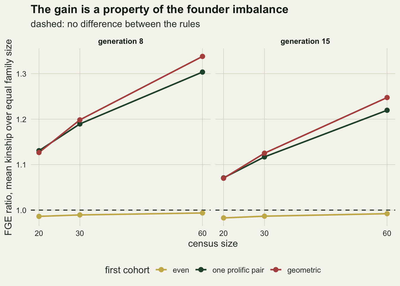
The grid repeats the pattern. With even founders the ratio lies between 0.983 and 0.994. With either uneven founder pattern it is at least 1.07 at every census size and at both horizons, the largest value being 1.34 at a census of 60 in generation 8. A larger population drifts more slowly, so the founder imbalance is a larger share of what it has to lose, and the rule that repairs the imbalance gains more.
Inbreeding and gene diversity are different targets
f_ev <- sapply(rules, function(r) f_at(r, "even", 30, 8)["mean"])
f_sk <- sapply(rules, function(r) f_at(r, "one_pair", 30, 8)["mean"])
names(f_ev) <- rules; names(f_sk) <- rules

drop_df <- do.call(rbind, lapply(seq_len(nrow(cells)), function(i) do.call(rbind,
  lapply(c(8, 15), function(g) data.frame(
    ped_gd = 1 - mean(sims[[i]][g, 1, ]), drop_gd = mean(sims[[i]][g, 4, ]),
    ped_ho = 1 - mean(sims[[i]][g, 3, ]), drop_ho = mean(sims[[i]][g, 6, ]),
    alleles = mean(sims[[i]][g, 5, ]), gen = g, rule = cells$rule[i])))))
drop_gap <- max(abs(drop_df$drop_gd - drop_df$ped_gd))
ho_gap   <- max(abs(drop_df$drop_ho - drop_df$ped_ho))
all_ev_mk  <- mean(sims[[cell_id("mk", "even", 30)]][8, 5, ])
all_ev_rnd <- mean(sims[[cell_id("random", "even", 30)]][8, 5, ])
Kin avoidance does exactly what it says. With even founders the mean inbreeding of the generation eight cohort is 0.090 under equal family sizes with random pairing and 0.073 under kin avoidance, and the mean kinship rule, whose pairing step also refuses close relatives, gives 0.072. None of that lower inbreeding came with more founder genome equivalents. With the prolific pair the mean kinship rule has the lowest inbreeding, 0.076 against 0.102 for kin avoidance, because it has the most diversity to draw unrelated mates from. Inbreeding is a property of this generation’s pairs and gene diversity is a property of the whole population, and a rule aimed at the first does not deliver the second.
The kinship matrix is an expectation over Mendelian sampling, and the gene drop run alongside it tests whether real genes follow. Over all 36 cells and both horizons the gene diversity of the dropped founder alleles differs from the pedigree value by at most 0.009, and the observed heterozygosity differs from one minus the mean pedigree inbreeding by at most 0.021. With a census of thirty and even founders the generation eight cohort still carries 12.9 of the twenty founder alleles on average under the mean kinship rule and 9.9 under random breeding.
fi_df <- do.call(rbind, lapply(which(cells$n_pop == 30), function(i) data.frame(
  fge = mean(sims[[i]][8, 2, ]), f = mean(sims[[i]][8, 3, ]),
  rule = factor(rule_lab[cells$rule[i]], levels = rule_lab),
  skew = factor(cells$skew[i], levels = names(first_cohort),
                labels = c("even", "one prolific pair", "geometric")))))
p_left <- ggplot(fi_df, aes(fge, f, colour = rule, shape = skew)) +
  geom_point(size = 3.2, stroke = 1.1) +
  scale_colour_manual(values = rule_cols, name = NULL) +
  scale_shape_manual(values = c(16, 17, 1), name = NULL) +
  guides(colour = guide_legend(nrow = 2), shape = guide_legend(nrow = 1)) +
  labs(x = "founder genome equivalents", y = "mean inbreeding coefficient",
       title = "Low F is not high FGE") +
  theme_datasheet() +
  theme(legend.position = "bottom", legend.box = "vertical")
p_right <- ggplot(drop_df, aes(ped_gd, drop_gd)) +
  geom_abline(slope = 1, intercept = 0, linetype = "dashed", colour = te_rust, linewidth = 0.6) +
  geom_point(colour = te_forest, size = 2, alpha = 0.8) +
  labs(x = "pedigree gene diversity", y = "gene drop gene diversity",
       title = "Genes follow the matrix") +
  coord_equal() +
  theme_datasheet()
(p_left | p_right) + plot_layout(widths = c(1.3, 1)) +
  plot_annotation(theme = theme_datasheet())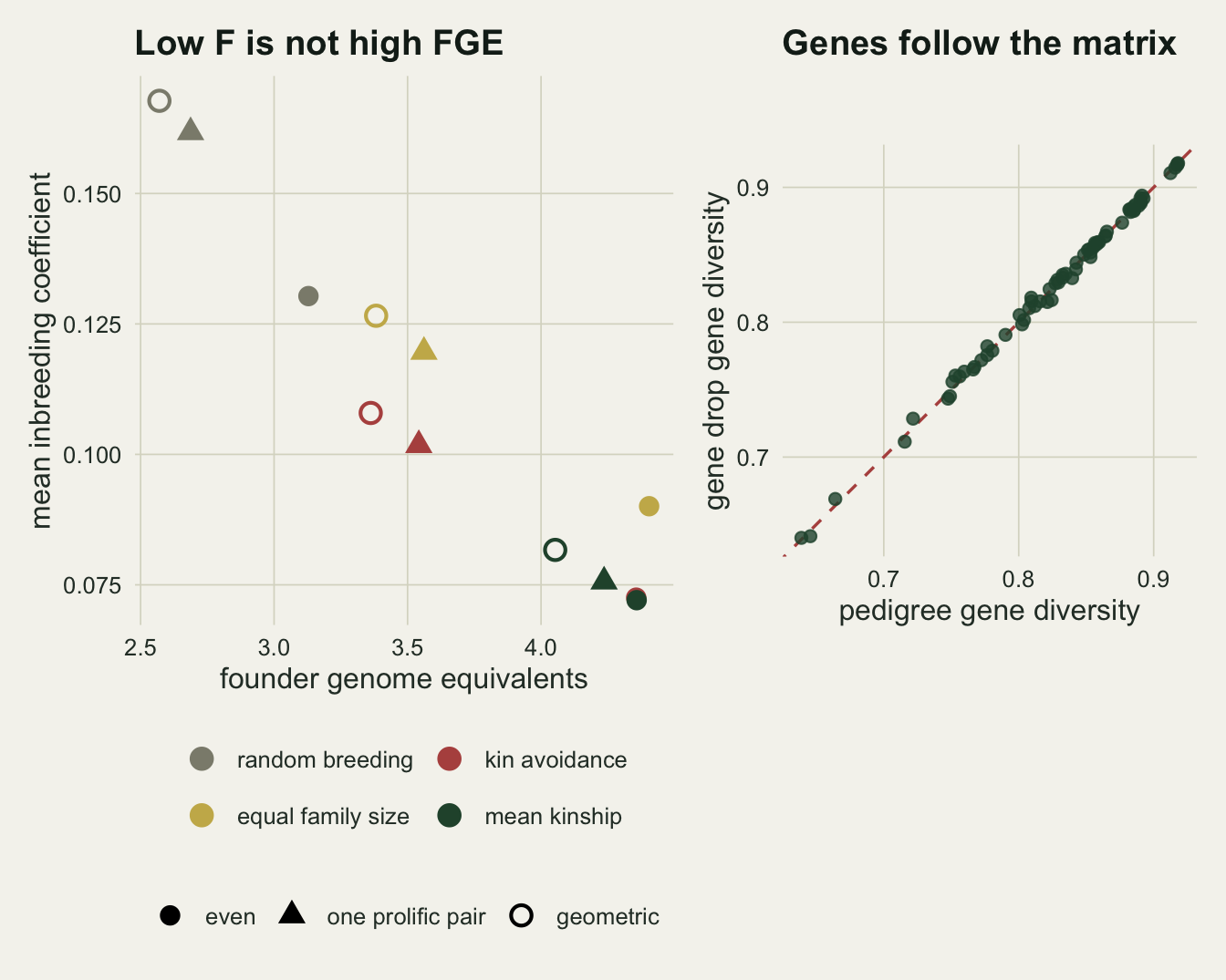
Unknown sires: a founder or an average
Real studbooks have holes. Group housing, a male introduced for a few days, a second male in the enclosure: some young have a recorded dam and a sire who is one of several males, or simply unknown. The convenient way to close such a hole records each unknown sire as a new founder, unrelated to everyone. The alternative averages kinship over the males that could have sired the young; Lacy set out in 2012 how the PMx software extends kinship calculations to uncertain parentage of this kind. The simulation below runs both on the prolific pair scenario with a census of thirty for eight generations, 150 lines per cell. Each young bred from generation two on has its sire unrecorded with probability u; its true sire is drawn uniformly from a candidate list made of the social mate plus one or two other breeding males, or all breeding males. The true kinship matrix is carried alongside the recorded one, and decisions use only the recorded one.
Four managements are compared at each u: the mean kinship rule with known parentage (as if every young had been genotyped), the mean kinship rule on the averaged record, the mean kinship rule on the phantom founder record, and equal family sizes, which ignore the record. Because extra-pair paternity itself changes the population, each convention is compared with the known parentage run and with equal family sizes at the same u, never with the u of zero.
run_studbook <- function(u, n_cand, mgmt, n_pop = 30, n_gen = 8) {
  k_true <- kin_found; k_avg <- k_true; k_ph <- k_true
  is_male <- rep(c(TRUE, FALSE), n_found / 2)
  pairs <- cbind(which(is_male), which(!is_male)); cnt <- first_cohort$one_pair
  for (g in seq_len(n_gen)) {
    if (g > 1) {
      k_use <- switch(mgmt, known = , efs = k_true, average = k_avg, phantom = k_ph)
      if (mgmt == "efs") {
        pairs <- pair_random(k_use, is_male); cnt <- alloc_equal(nrow(pairs), n_pop)
      } else {
        pairs <- pair_mk(k_use, is_male); cnt <- alloc_greedy(k_use, pairs, n_pop)
      }
    }
    fam <- rep(seq_len(nrow(pairs)), cnt); n_off <- length(fam); n_par <- nrow(k_true)
    social <- pairs[fam, 1]; breeders <- unique(pairs[cnt > 0, 1])
    unk <- if (g > 1) runif(n_off) < u else rep(FALSE, n_off)
    dam_w <- matrix(0, n_off, n_par); dam_w[cbind(seq_len(n_off), pairs[fam, 2])] <- 1
    sire_true <- social
    avg_w <- matrix(0, n_off, n_par); avg_w[cbind(seq_len(n_off), social)] <- 1
    for (i in which(unk)) {
      others <- breeders[breeders != social[i]]
      cand <- if (n_cand - 1 >= length(others)) c(social[i], others) else
        c(social[i], others[sample.int(length(others), n_cand - 1)])
      sire_true[i] <- cand[sample.int(length(cand), 1)]
      avg_w[i, ] <- 0; avg_w[i, cand] <- 1 / length(cand)
    }
    true_w <- matrix(0, n_off, n_par); true_w[cbind(seq_len(n_off), sire_true)] <- 1
    k_true <- next_kinship(k_true, dam_w, true_w)$kin
    k_avg  <- next_kinship(k_avg, dam_w, avg_w)$kin
    n_ph <- sum(unk)
    ph_w <- true_w
    k_x  <- k_ph
    if (n_ph) {
      k_x <- matrix(0, n_par + n_ph, n_par + n_ph); k_x[1:n_par, 1:n_par] <- k_ph
      diag(k_x)[n_par + seq_len(n_ph)] <- 0.5
      dam_w <- cbind(dam_w, matrix(0, n_off, n_ph))
      ph_w  <- cbind(true_w, matrix(0, n_off, n_ph)); ph_w[unk, ] <- 0
      ph_w[cbind(which(unk), n_par + seq_len(n_ph))] <- 1
    }
    k_ph <- next_kinship(k_x, dam_w, ph_w)$kin
    is_male <- sample(rep(c(TRUE, FALSE), length.out = n_off))
  }
  c(true = fge_of(k_true), average = fge_of(k_avg), phantom = fge_of(k_ph))
}

n_rep_sire <- 150
u_grid     <- c(0, 0.1, 0.25, 0.5)
cand_grid  <- c(2, 3, 99)
mgmt_set   <- c("known", "average", "phantom", "efs")
sire_cells <- expand.grid(u = u_grid, n_cand = cand_grid, mgmt = mgmt_set,
                          stringsAsFactors = FALSE)
sire_cells <- sire_cells[!(sire_cells$u == 0 & (sire_cells$n_cand != 99 |
                           sire_cells$mgmt %in% c("average", "phantom"))), ]
set.seed(4142)
sire_out <- t(sapply(seq_len(nrow(sire_cells)), function(i) {
  v <- replicate(n_rep_sire, run_studbook(sire_cells$u[i], sire_cells$n_cand[i], sire_cells$mgmt[i]))
  c(rowMeans(v), se = sd(v["true", ]) / sqrt(n_rep_sire))
}))
sire_res <- cbind(sire_cells, sire_out)
sire_get <- function(u, n_cand, mgmt, col = "true") {
  if (u == 0) { n_cand <- 99; if (mgmt != "efs") mgmt <- "known" }
  sire_res[sire_res$u == u & sire_res$n_cand == n_cand & sire_res$mgmt == mgmt, col]
}
kept_share <- function(u, n_cand, mgmt) {
  (sire_get(u, n_cand, mgmt) - sire_get(u, n_cand, "efs")) /
    (sire_get(u, n_cand, "known") - sire_get(u, n_cand, "efs"))
}
share_tab <- sapply(c(0.1, 0.25, 0.5), function(u)
  c(avg = kept_share(u, 99, "average"), ph = kept_share(u, 99, "phantom")))
infl_ph  <- sapply(c(0.1, 0.25, 0.5), function(u) sire_get(u, 99, "phantom", "phantom") / sire_get(u, 99, "phantom"))
infl_avg <- sapply(c(0.1, 0.25, 0.5), function(u) sire_get(u, 99, "average", "average") / sire_get(u, 99, "average"))
max_se_sire <- max(sire_res$se)
drop_u <- sapply(c("known", "efs", "phantom"), function(mg) sire_get(0.1, 99, mg) - sire_get(0.5, 99, mg))
Start with what the studbook reports. With all breeding males as candidates and a quarter of sires unknown, the phantom founder record under mean kinship management reports an FGE of 12.06 when the true value is 3.55, 3.4 times too high; at a tenth of sires unknown the ratio is 2.1 and at a half 5.0. That inflation is bookkeeping: every phantom is one more unrelated founder in the arithmetic. The averaged record reports 3.91 against a true 3.92, and its ratio of reported to true FGE stays between 0.9986 and 1.0005 across the three rates.
The decision cost is the number that needs the simulation. At a quarter unknown, all males as candidates, known parentage keeps a true FGE of 3.94 and equal family sizes 3.32; the averaged record keeps 3.92 and the phantom record 3.55. Measured as a share of the gap between equal families and known parentage at the same rate, averaging keeps 96 per cent of the mean kinship advantage and the phantom convention 37 per cent. At a tenth unknown the shares are 98 and 29 per cent, and at a half 86 and 53 per cent; the largest standard error of any true FGE in this grid is 0.016. Between a tenth and a half unknown the phantom run’s true FGE falls by 0.14, less than half as far as under known parentage (0.33) and just over half as far as under equal family sizes (0.26), which is why its share recovers at the higher rates. The phantom convention does its harm early: young with a phantom sire look unrelated to everyone, the greedy allocation favours them, and a few unknown sires are enough to steer breeding towards whichever lines they happened to land in.
mgmt_lab <- c(known = "mean kinship, parentage known", average = "mean kinship, averaged sires",
              phantom = "mean kinship, phantom founders", efs = "equal family size")
cand_lab <- c(`2` = "2 candidates", `3` = "3 candidates", `99` = "all breeding males")
sire_plot <- do.call(rbind, lapply(cand_grid, function(nc) do.call(rbind,
  lapply(mgmt_set, function(mg) data.frame(u = u_grid, n_cand = nc, mgmt = mg,
    fge = sapply(u_grid, function(u) sire_get(u, nc, mg)))))))
sire_plot$mgmt   <- factor(mgmt_lab[sire_plot$mgmt], levels = mgmt_lab)
sire_plot$n_cand <- factor(cand_lab[as.character(sire_plot$n_cand)], levels = cand_lab)
mgmt_cols <- setNames(c(te_forest, te_gold, te_rust, "#8c8b7c"), mgmt_lab)
p_true <- ggplot(sire_plot, aes(u, fge, colour = mgmt)) +
  geom_line(linewidth = 0.9) +
  geom_point(size = 2) +
  facet_wrap(~ n_cand, ncol = 1) +
  scale_colour_manual(values = mgmt_cols, name = NULL) +
  scale_x_continuous(breaks = u_grid) +
  labs(x = "share of sires unknown", y = "true founder genome equivalents",
       title = "True diversity kept") +
  theme_datasheet() +
  theme(legend.position = "bottom", legend.direction = "vertical",
        strip.text = element_text(colour = te_ink, face = "bold"))
infl_df <- data.frame(u = rep(c(0.1, 0.25, 0.5), 2), ratio = c(infl_ph, infl_avg),
                      conv = rep(c("phantom founders", "averaged sires"), each = 3))
p_infl <- ggplot(infl_df, aes(u, ratio, colour = conv)) +
  geom_hline(yintercept = 1, linetype = "dashed", colour = te_body, linewidth = 0.6) +
  geom_line(linewidth = 0.9) +
  geom_point(size = 2.4) +
  scale_colour_manual(values = c(te_gold, te_rust), name = NULL) +
  scale_x_continuous(breaks = c(0.1, 0.25, 0.5)) +
  scale_y_continuous(limits = c(0, NA)) +
  labs(x = "share of sires unknown", y = "reported FGE over true FGE",
       title = "What the studbook says") +
  theme_datasheet() +
  theme(legend.position = "bottom", legend.direction = "vertical")
(p_true | p_infl) + plot_layout(widths = c(1.2, 1)) +
  plot_annotation(theme = theme_datasheet())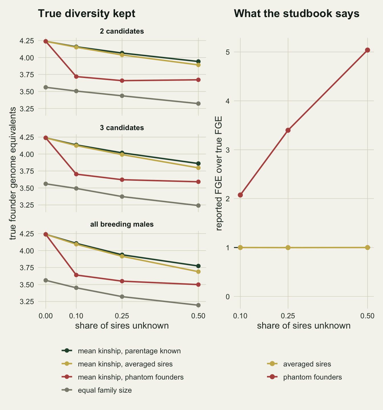
What to report
Report the founder representation of the first cohorts, not only the number of founders. The simulations here say that the choice between equal family sizes and mean kinship management is worth arguing about only when a few founders dominate the early studbook, and the founder genome equivalents of the current population, set beside the number of founders, is the direct measure of that imbalance: ten founders with an FGE near 5.8 after one generation is a programme where the ranking rule matters.
State the rule in full. “Managed by mean kinship” covers pairing by rank with or without a kinship ceiling, and allocation of young by rank, by change in mean kinship, or by an explicit optimisation. In these runs the allocation carried about nine tenths of the advantage and the pairing almost none, so a programme that pairs by mean kinship but lets every pair breed equally is running equal family sizes.
Give gene diversity and FGE together. The ninety per cent target is written in gene diversity, and on that scale the generation eight gap between the rules with a prolific founder pair was 2.2 percentage points, from 0.860 to 0.882; the same gap is 0.67 founder genome equivalents, 19 per cent more founders’ worth of genes. A reader who sees only the first number will think the rules are equivalent.
Say how unknown sires were recorded, what share of the young they affect, and report FGE under both conventions if the studbook uses phantom founders. The averaged record reported its own true FGE to within 0.14 per cent here, whereas the phantom record overstated it several times over, and that overstatement then fed the breeding decisions.
Honest limits
Generations are discrete. Every animal breeds once and leaves; real captive populations of long-lived species keep founders and early offspring alive and breeding for decades, and the mean kinship rule can then use a living under-represented founder directly. Whether the skew advantage is larger or smaller with overlapping generations was not simulated, and the fifteen generation horizon here is hundreds of years for many zoo species.
The mean kinship rule is a stand-in for what PMx and similar software do, not a copy. Those tools rank by mean kinship, score candidate pairs by the difference in mean kinship between the partners and by the inbreeding of their young, and leave the numbers of young to husbandry targets set by the keeper. The greedy allocation used here is closer to optimal contribution selection and is more aggressive than a keeper would be: in generation two it gave 12 per cent of pairs no young at all. A softer allocation would be expected to keep less of the gain from an uneven start.
The census is fixed, every animal is fertile, sexes are exactly balanced and every planned pairing succeeds. Real programmes lose pairings to incompatibility, age and transport, and those failures fall hardest on the rarest animals.
The founders are unrelated and not inbred. Wild-caught founders taken from the same place are often related, and treating them as unrelated inflates FGE in the same way the phantom sires do; that problem is not tested here.
Unknown sires are drawn uniformly from the candidate list, independently for each young. In group housing a dominant male usually sires most of the young, and siblings in a litter usually share a sire, so a real candidate list carries more information than a uniform average uses and the phantom convention may do less or more damage than measured. The averaged record was unbiased here partly because the simulation’s truth matched the convention’s assumption.
The comparison is about neutral genetic diversity. None of the rules addresses adaptation to captivity, inbreeding depression beyond its kinship arithmetic, or demographic stability, which are also part of what a studbook keeper manages.
References
Lacy RC 1995 Zoo Biology 14(6):565-577 (10.1002/zoo.1430140609)
Montgomery ME, Ballou JD, Nurthen RK, England PR, Briscoe DA, Frankham R 1997 Zoo Biology 16(5):377-389 (10.1002/(SICI)1098-2361(1997)16:5<377::AID-ZOO1>3.0.CO;2-7)
Meuwissen THE 1997 Journal of Animal Science 75(4):934-940 (10.2527/1997.754934x)
Lacy RC 2012 Journal of Heredity 103(2):197-205 (10.1093/jhered/esr135)