library(ggplot2)

te_pal <- list(forest = "#275139", green = "#2f8f63", sage = "#93a87f",
               clay = "#b5534e", gold = "#cda23f", line = "#dad9ca",
               ink = "#16241d", paper = "#f5f4ee")

theme_te <- function() {
  theme_minimal(base_size = 12) +
    theme(panel.grid.minor = element_blank(),
          panel.grid.major = element_line(colour = "#e7e6dc"),
          plot.background = element_rect(fill = "#f5f4ee", colour = NA),
          panel.background = element_rect(fill = "#f5f4ee", colour = NA),
          plot.title = element_text(face = "bold", colour = te_pal$ink),
          axis.title = element_text(colour = "#2c3a31"),
          legend.position = "bottom")
}Checking an animal model
R
quantitative genetics
heritability
model checking
ecology tutorial
Four measured checks on a fitted animal model in R: pedigree errors, the fixed-effect denominator, evolvability, and the boundary at zero in wild populations.
The nest box scheme has been running for nineteen years. Every chick is ringed before fledging, every breeding female is caught on the nest, and the ring numbers have been typed into the same spreadsheet since the second field season. Out of that comes a pedigree: a few thousand individuals, mothers known for almost all of them, fathers taken from the male seen feeding at the box. Someone fits an animal model to tarsus length and a heritability comes back, somewhere around a third, which is exactly where a skeletal trait in a passerine is supposed to be.
That number is now going to be repeated. It will go into a talk, then into a discussion section, then into a table in somebody else’s meta-analysis, where it will sit beside a value from a different species measured in a different way. By the time it gets there, nobody remembers that the fathers were social fathers, that the model had sex and hatch date in it, or that the confidence interval was wide enough to hold half the values anybody has ever published for a skeletal trait.
None of that is fraud or even sloppiness. It is the ordinary fate of a summary statistic that travels further than its methods section. The animal model is a good tool and the estimate is usually computed correctly. The problem is that a heritability is a ratio of two quantities, and almost everything that can go wrong with it goes wrong quietly: the estimate still comes back, it still looks plausible, and nothing in the output complains.
This post is the closing diagnostic for the animal model cluster. It runs four checks on a fitted animal model, and every one of them is a measurement against a truth we set ourselves, in a simulation where we know the answer. Each check can change what you would report. Two of them change the number itself, one changes which summary you should report at all, and one changes the test you attach to it.
The pattern of the post is the same one used everywhere else on this blog: predict, then measure, then keep the measurement. Three of the expectations below did not survive the measurement, one of them wrong by a factor close to two, and the sections around them have been rebuilt on what the simulation actually did rather than on what the arithmetic said it should do.
The three companion posts build the pieces used here: The animal model in R constructs the relationship matrix and the restricted maximum likelihood fitter, Pedigree structure and heritability precision measures how the shape of the pedigree sets the sampling error, and Maternal effects inflate heritability measures the bias from a shared environment. This post is self contained: the pedigree simulator, the relationship matrix and the fitter are written again below, compactly, so you can run it on its own.
The pedigree, the relationship matrix and the fitter
The population is a small caricature of a passerine study. A founder generation of unrelated adults produces two cohorts of offspring; males differ in mating success, so the offspring generations contain paternal half sibs as well as full sibs and maternal half sibs. Every individual gets a phenotype, founders included.
The relationship matrix is built by the recursive rule that everyone learns and nobody enjoys writing out: an individual’s relatedness to an earlier individual is the average of its two parents’ relatedness to that individual, and its own diagonal entry is one plus half the relatedness between its parents. Unknown parents point at a padding row of zeros.
make_pedigree <- function(n_sire, n_dam, n_off, n_gen) {
  sire <- rep(0L, n_sire + n_dam)
  dam <- rep(0L, n_sire + n_dam)
  sexv <- c(rep(1L, n_sire), rep(0L, n_dam))
  gen <- rep(0L, n_sire + n_dam)
  cur_m <- seq_len(n_sire)
  cur_f <- n_sire + seq_len(n_dam)
  pools <- list()
  for (g in seq_len(n_gen)) {
    pools[[g]] <- cur_m
    success <- rgamma(length(cur_m), shape = 1.2, rate = 1.2)
    s_new <- sample(cur_m, n_off, replace = TRUE, prob = success)
    d_new <- sample(cur_f, n_off, replace = TRUE)
    new_id <- length(sire) + seq_len(n_off)
    sire <- c(sire, s_new)
    dam <- c(dam, d_new)
    sx <- rbinom(n_off, 1, 0.5)
    sexv <- c(sexv, sx)
    gen <- c(gen, rep(g, n_off))
    cur_m <- new_id[sx == 1L]
    cur_f <- new_id[sx == 0L]
  }
  list(sire = sire, dam = dam, sex = sexv, gen = gen, pools = pools)
}

make_A <- function(sire, dam) {
  nn <- length(sire)
  out <- matrix(0, nn + 1L, nn + 1L)
  s <- ifelse(sire == 0L, nn + 1L, sire)
  d <- ifelse(dam == 0L, nn + 1L, dam)
  for (i in seq_len(nn)) {
    if (i > 1L) {
      j <- seq_len(i - 1L)
      v <- 0.5 * (out[j, s[i]] + out[j, d[i]])
      out[i, j] <- v
      out[j, i] <- v
    }
    out[i, i] <- 1 + 0.5 * out[s[i], d[i]]
  }
  out[seq_len(nn), seq_len(nn)]
}

set.seed(20260727)
ped <- make_pedigree(n_sire = 30, n_dam = 60, n_off = 120, n_gen = 2)
n_ind <- length(ped$sire)
amat <- make_A(ped$sire, ped$dam)
ev_true <- eigen(amat, symmetric = TRUE)
lower <- lower.tri(amat)

print(round(c(founding_sires = 30, founding_dams = 60, offspring_per_cohort = 120,
              cohorts = 2, individuals = n_ind,
              with_a_recorded_sire = sum(ped$sire > 0)), 4))
founding_sires founding_dams offspring_per_cohort
30 60 120
cohorts individuals with_a_recorded_sire
2 330 240 print(round(c(mean_diagonal = mean(diag(amat)),
largest_relatedness = max(amat[lower]),
pairs_related_at_all = mean(amat[lower] > 0),
smallest_eigenvalue = min(ev_true$values)), 4)) mean_diagonal largest_relatedness pairs_related_at_all
1.0064 0.6250 0.1422
smallest_eigenvalue
0.0489 The pedigree holds 330 individuals, of whom 240 have a recorded sire. The mean diagonal of the relationship matrix is 1.0064, so there is a trace of inbreeding but not much: the founders were unrelated and only two cohorts have been produced. The largest off-diagonal entry is 0.625, which is a parent and its offspring in a family whose two parents are themselves related, so the offspring carries a little inbreeding of its own, and 0.1422 of all pairs have any relatedness at all. The smallest eigenvalue is 0.0489, comfortably positive, which matters for the trick used next.
The fitter is restricted maximum likelihood, written out by hand. The model is \(y = X\beta + u + e\) with \(u \sim N(0, A\sigma^2_a)\) and \(e \sim N(0, I\sigma^2_e)\), so the phenotypic covariance is \(V = A\sigma^2_a + I\sigma^2_e\). Two things make this fast enough to run several hundred times in a post. First, the residual variance can be profiled out analytically, leaving a one dimensional search over the heritability itself. Second, the eigendecomposition of \(A\) can be computed once and reused: writing \(A = Q\Lambda Q'\) and \(V = \sigma^2_e Q(\Lambda g + I)Q'\) with \(g = \sigma^2_a/\sigma^2_e\) turns every determinant and every solve into an operation on a vector.
reml <- function(y, X, ev) {
  lam <- ev$values
  ys <- as.vector(crossprod(ev$vectors, y))
  xs <- crossprod(ev$vectors, X)
  nn <- length(y)
  pp <- ncol(X)
  core <- function(h2) {
    g <- h2 / (1 - h2)
    dd <- g * lam + 1
    kiy <- ys / dd
    xkx <- crossprod(xs, xs / dd)
    xky <- crossprod(xs, kiy)
    ch <- chol(xkx)
    bb <- backsolve(ch, backsolve(ch, xky, transpose = TRUE))
    ss <- sum(ys * kiy) - sum(xky * bb)
    list(ll = -0.5 * ((nn - pp) * log(ss / (nn - pp)) + sum(log(dd)) +
                        2 * sum(log(diag(ch)))),
         ve = ss / (nn - pp), g = g)
  }
  at_zero <- core(0)
  best <- optimize(function(h2) core(h2)$ll, c(0, 0.999), maximum = TRUE, tol = 1e-7)
  h2hat <- if (best$objective > at_zero$ll) best$maximum else 0
  fit <- core(h2hat)
  list(h2 = h2hat, va = fit$g * fit$ve, ve = fit$ve, vp = fit$g * fit$ve + fit$ve,
       ll = fit$ll, ll_zero = at_zero$ll, lrt = max(0, 2 * (fit$ll - at_zero$ll)))
}

chol_a <- ev_true$vectors %*% diag(sqrt(pmax(ev_true$values, 0)))
breeding_values <- function(va) as.vector(chol_a %*% rnorm(n_ind)) * sqrt(va)

set.seed(20260801)
sexf <- ped$sex
x_sex <- cbind(1, sexf)
y_demo <- 10 + 2 * sexf + breeding_values(1) + rnorm(n_ind, 0, 1)
demo <- reml(y_demo, x_sex, ev_true)
print(round(c(true_h2 = 0.5, estimated_h2 = demo$h2,
              true_va = 1, estimated_va = demo$va,
              true_ve = 1, estimated_ve = demo$ve), 4))
true_h2 estimated_h2 true_va estimated_va true_ve estimated_ve
0.5000 0.5141 1.0000 1.1182 1.0000 1.0569 On one data set simulated with an additive variance of 1 and a residual variance of 1, so a true heritability of 0.5, the fitter returns 0.5141, with an additive variance of 1.1182 and a residual variance of 1.0569. That is the machinery working. Everything below uses this same fitter and this same pedigree, so any difference between sections comes from the thing being checked and not from a change of tools.
A word on why the search is over the heritability rather than over the two variances. The constrained maximum has to be allowed to sit exactly on the boundary at zero, because that is the subject of the fourth check. Searching over an interval that includes zero, and then comparing the best interior value against the value exactly at zero, gives a point mass at zero that a gradient method with a soft lower bound would smear out.
Check one: is the pedigree right
Wild pedigrees are wrong in a specific way. Mothers are usually safe, because someone watched the female sitting on the eggs. Fathers are the social fathers, and in many passerines a tenth or more of the chicks are sired by a male from another territory. The recorded pedigree therefore has correct dam links and a fraction of wrong sire links.
The prediction before measuring: if a fraction \(p\) of sire links is wrong, then a fraction \(p\) of the paternal relatedness is destroyed, so the estimated heritability should be attenuated to \((1-p)\) times the truth. This is the arithmetic everybody does in their head, and it is the reason people quote a correction of “add a bit for extra-pair paternity”.
The simulation corrupts sires only. For a chosen error rate, that fraction of individuals with a recorded sire has the sire replaced by another male from the same cohort of candidate fathers, which is what a social father is: a plausible male who was there. Phenotypes are always generated from the true pedigree; the model is always fitted with the corrupted one. Eight independent error realisations per rate, four phenotype replicates each, so thirty-two fits per rate.
corrupt_sires <- function(pedigree, p) {
  s <- pedigree$sire
  idx <- which(s > 0L)
  k <- round(p * length(idx))
  if (k > 0) {
    for (i in sample(idx, k)) {
      pool <- pedigree$pools[[pedigree$gen[i]]]
      alt <- pool[pool != s[i]]
      s[i] <- alt[sample.int(length(alt), 1L)]
    }
  }
  s
}

set.seed(20260729)
rates <- c(0, 0.1, 0.2, 0.3, 0.4)
n_err <- 8
n_phen <- 4
a_true <- amat[lower]
rows <- list()
k <- 0
for (p in rates) {
  for (e in seq_len(n_err)) {
    a_bad <- make_A(corrupt_sires(ped, p), ped$dam)
    ev_bad <- eigen(a_bad, symmetric = TRUE)
    a_off <- a_bad[lower]
    attn <- cov(a_true, a_off) / var(a_off)
    for (r in seq_len(n_phen)) {
      y <- 10 + 2 * sexf + breeding_values(1) + rnorm(n_ind, 0, 1)
      f_bad <- reml(y, x_sex, ev_bad)
      f_ok <- reml(y, x_sex, ev_true)
      k <- k + 1
      rows[[k]] <- c(rate = p, attn = attn, h2_bad = f_bad$h2, h2_ok = f_ok$h2,
                     gap = f_ok$ll - f_bad$ll)
    }
  }
}
err_res <- as.data.frame(do.call(rbind, rows))

err_tab <- data.frame(
  error_rate = rates,
  h2_recorded = as.vector(tapply(err_res$h2_bad, err_res$rate, mean)),
  h2_true_ped = as.vector(tapply(err_res$h2_ok, err_res$rate, mean)),
  se_recorded = as.vector(tapply(err_res$h2_bad, err_res$rate,
                                 function(z) sd(z) / sqrt(length(z)))),
  naive_pred = as.vector(tapply(err_res$h2_ok, err_res$rate, mean)) * (1 - rates),
  attenuation = as.vector(tapply(err_res$attn, err_res$rate, mean)))
err_tab$eiv_pred <- err_tab$h2_true_ped * err_tab$attenuation
print(round(err_tab, 4))
error_rate h2_recorded h2_true_ped se_recorded naive_pred attenuation
1 0.0 0.5120 0.5120 0.0194 0.5120 1.0000
2 0.1 0.4779 0.5103 0.0181 0.4593 0.9345
3 0.2 0.4455 0.4938 0.0148 0.3951 0.8609
4 0.3 0.3873 0.4535 0.0152 0.3175 0.8046
5 0.4 0.3765 0.4894 0.0193 0.2936 0.7311
eiv_pred
1 0.5120
2 0.4769
3 0.4251
4 0.3649
5 0.3578print(round(c(replicates_per_rate = n_err * n_phen,
observed_ratio_at_0.4 = err_tab$h2_recorded[5] / err_tab$h2_true_ped[5],
naive_ratio_at_0.4 = 1 - 0.4,
attenuation_at_0.4 = err_tab$attenuation[5]), 4)) replicates_per_rate observed_ratio_at_0.4 naive_ratio_at_0.4
32.0000 0.7693 0.6000
attenuation_at_0.4
0.7311 The heritability does fall with the error rate, in the direction predicted. At a sire error rate of 0.4 the mean estimate from the recorded pedigree is 0.3765 against 0.4894 from the true pedigree, a ratio of 0.7693. The prediction was 0.6. The estimate kept more of its value than the arithmetic said it would: the loss the errors actually caused is a little over half the loss that was predicted, and this is the result the section had to be rebuilt around.
The reason is visible in the relationship matrix itself, and it is the oldest result in measurement error theory. What the fitter does, in effect, is regress phenotypic products on recorded relatedness. When the predictor carries error, the fitted coefficient is attenuated by the regression of the true predictor on the recorded one, which is not the same as the fraction of entries that were changed. The column attenuation in the table above is exactly that coefficient, computed from the two relationship matrices with no phenotypes involved: 0.7311 at an error rate of 0.4, against 0.6 for the naive version. The measured ratio, 0.7693, sits nearer the first than the second.
Corrupting a sire link does not zero the relatedness between the affected pairs. The wrong sire is another male from the same cohort, so he is often a relative of the true sire, and every dam link is still correct, so maternal half sibs and full sibs keep their maternal share. The recorded matrix is a noisy version of the true one, not a diluted one, and noise in a predictor attenuates by a factor you have to compute rather than guess.
lines_dat <- rbind(
  data.frame(rate = rates, value = err_tab$h2_recorded, series = "recorded pedigree"),
  data.frame(rate = rates, value = err_tab$h2_true_ped, series = "true pedigree"),
  data.frame(rate = rates, value = err_tab$naive_pred, series = "naive (1 - p) prediction"),
  data.frame(rate = rates, value = err_tab$eiv_pred, series = "errors-in-variables prediction"))
lines_dat$series <- factor(lines_dat$series,
                           levels = c("recorded pedigree", "true pedigree",
                                      "naive (1 - p) prediction",
                                      "errors-in-variables prediction"))
bars_dat <- data.frame(rate = rates,
                       lo = err_tab$h2_recorded - err_tab$se_recorded,
                       hi = err_tab$h2_recorded + err_tab$se_recorded)

ggplot(lines_dat, aes(rate, value, colour = series, linetype = series)) +
  geom_line(linewidth = 0.9) +
  geom_errorbar(data = bars_dat, inherit.aes = FALSE,
                aes(x = rate, ymin = lo, ymax = hi), width = 0.012,
                colour = te_pal$clay, linewidth = 0.7) +
  geom_point(size = 2.4) +
  scale_colour_manual(values = c(te_pal$clay, te_pal$forest, te_pal$gold, te_pal$sage),
                      name = NULL) +
  scale_linetype_manual(values = c("solid", "solid", "dashed", "dashed"), name = NULL) +
  labs(x = "fraction of sire links that are wrong",
       y = "heritability estimate",
       title = "Wrong sires attenuate less than proportionally") +
  guides(colour = guide_legend(nrow = 2), linetype = guide_legend(nrow = 2)) +
  theme_te() +
  theme(plot.margin = margin(6, 14, 6, 6))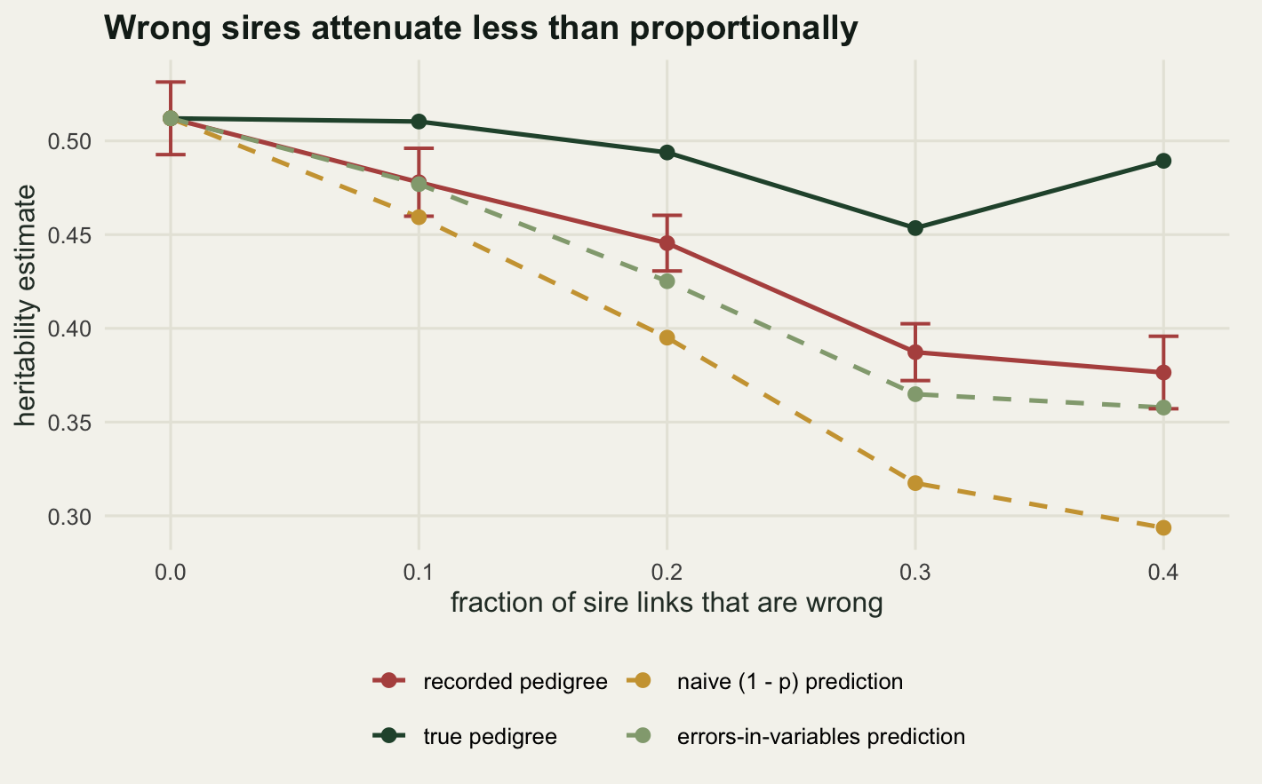
The second question about pedigree error is whether you could catch it from the phenotypes. The fits above give a direct answer, because each replicate was fitted twice, once with the true pedigree and once with the corrupted one, on identical data. The difference in maximised restricted likelihood is a measure of how much better the true pedigree explains the phenotypes.
detect <- data.frame(
  error_rate = rates,
  mean_loglik_gap = as.vector(tapply(err_res$gap, err_res$rate, mean)),
  prop_gap_above_2 = as.vector(tapply(err_res$gap, err_res$rate, function(z) mean(z > 2))),
  prop_wrong_ped_wins = as.vector(tapply(err_res$gap, err_res$rate, function(z) mean(z < 0))))
print(round(detect, 4))
error_rate mean_loglik_gap prop_gap_above_2 prop_wrong_ped_wins
1 0.0 0.0000 0.000 0.0000
2 0.1 1.9883 0.500 0.2188
3 0.2 3.9030 0.625 0.1875
4 0.3 5.5574 0.750 0.0625
5 0.4 7.3415 0.875 0.0312At a realistic error rate of 0.1 the true pedigree beats the corrupted one by 1.9883 log-likelihood units on average, and in 0.2188 of replicates the corrupted pedigree actually fits better. A gap of more than two units, which is the scale at which anyone would call a difference interesting, appears in 0.5 of replicates. At an error rate of 0.4 the picture is clearer, with a mean gap of 7.3415 units and 0.875 of replicates above two.
That comparison is not available to you. It required two pedigrees, one of them correct. In a real study you have one recorded pedigree and nothing to compare it against, and the likelihood of a single fitted model carries no interpretable signal on its own about whether the fathers are right. The check for pedigree error is molecular, not statistical: genotype a sample of broods, estimate the extra-pair rate, and then decide what to do about it. The measurement above tells you what to do with that rate once you have it, which is to correct by the errors-in-variables attenuation and not by \((1-p)\).
Check two: what the denominator is
Heritability is \(\sigma^2_a / V_P\) and the argument is almost always about the numerator. The denominator is where comparability actually breaks, because \(V_P\) in a fitted animal model is not the raw variance of the trait. It is the variance left after the fixed effects have taken their share. Put sex in the model and \(V_P\) loses the between-sex variance. Add a strong environmental covariate and it loses that too. The genetics have not changed and the heritability has.
Here is the same trait, simulated once and fitted three ways: with no fixed effects at all, with sex, and with sex plus a continuous environmental covariate that carries a real effect. Two hundred replicate data sets, all with an additive variance of 1 and a residual variance of 1.
set.seed(20260728)
n_rep_b <- 200
store <- matrix(NA_real_, n_rep_b, 9)
for (r in seq_len(n_rep_b)) {
  envq <- rnorm(n_ind)
  y <- 10 + 2 * sexf + 1.5 * envq + breeding_values(1) + rnorm(n_ind, 0, 1)
  f1 <- reml(y, matrix(1, n_ind, 1), ev_true)
  f2 <- reml(y, cbind(1, sexf), ev_true)
  f3 <- reml(y, cbind(1, sexf, envq), ev_true)
  store[r, ] <- c(f1$h2, f2$h2, f3$h2, f1$vp, f2$vp, f3$vp, f1$va, f2$va, f3$va)
}
mns <- colMeans(store)
ses <- apply(store, 2, function(z) sd(z) / sqrt(length(z)))

den_tab <- data.frame(
  fixed_effects = c("intercept only", "sex", "sex + environment"),
  h2 = mns[1:3], se_h2 = ses[1:3],
  v_p = mns[4:6], v_a = mns[7:9], se_v_a = ses[7:9],
  v_e = mns[4:6] - mns[7:9])
print(round(den_tab[, -1], 4))
h2 se_h2 v_p v_a se_v_a v_e
1 0.2190 0.0072 5.2375 1.1562 0.0399 4.0812
2 0.2285 0.0068 4.2422 0.9746 0.0303 3.2677
3 0.4910 0.0071 1.9888 0.9834 0.0175 1.0054print(round(c(replicates = n_rep_b,
variance_removed_by_sex = mns[4] - mns[5],
variance_removed_by_environment = mns[5] - mns[6],
numerator_movement = mns[7] - mns[9],
denominator_movement = mns[4] - mns[6],
h2_ratio_top_to_bottom = mns[3] / mns[1]), 4)) replicates variance_removed_by_sex
200.0000 0.9952
variance_removed_by_environment numerator_movement
2.2535 0.1729
denominator_movement h2_ratio_top_to_bottom
3.2487 2.2424 Three heritabilities from one data generating process, with no genetics changed: 0.219 with no fixed effects, 0.2285 with sex, and 0.491 with sex and the environmental covariate. The last is 2.2424 times the first. Any of the three could appear in a paper, correctly computed, with the same data behind it.
Most of that is the denominator. The phenotypic variance goes from 5.2375 to 1.9888: sex removes 0.9952 of variance, the environmental covariate removes another 2.2535, and the heritability more than doubles on the way down. The additive variance, which is the part people argue about, is 1.1562, 0.9746 and 0.9834 across the three models, so it moves by 0.1729 from the first model to the last while the denominator moves by 3.2487.
That numerator movement is not noise, and this is the second place where the simulation refused the tidy version of the story. The Monte Carlo standard errors on the three additive variances are 0.0399, 0.0303 and 0.0175, so the intercept-only estimate of 1.1562 is several standard errors above the other two and above the true value of 1. Dropping a fixed effect does not send all of its variance to the residual. Some of it can be picked up by the additive component, if the dropped covariate happens to look like a breeding value.
Whether it does is measurable, and it is a property of the covariate and the pedigree rather than a general law. A vector that is smooth across families, so that relatives share values, projects onto the same directions of the relationship matrix that additive genetic effects occupy. The quantity below is the ratio of a vector’s quadratic form under the relationship matrix to its own sum of squares, after centring, compared with the same ratio for random binary vectors of the same length on the same pedigree.
set.seed(20260804)
qform <- function(v) {
  v <- v - mean(v)
  sum(v * (amat %*% v)) / sum(v^2)
}
random_ref <- replicate(200, qform(rbinom(n_ind, 1, 0.5)))
align <- c(sex_vector = qform(sexf),
           random_binary_mean = mean(random_ref),
           random_binary_sd = sd(random_ref))
print(round(c(align, z_score = as.vector((align[1] - align[2]) / align[3]),
              reference_draws = 200), 4))
sex_vector random_binary_mean random_binary_sd z_score
1.1508 0.9982 0.1045 1.4605
reference_draws
200.0000 n_probe <- 16
n_rep_probe <- 20
probe <- data.frame(alignment = numeric(n_probe), v_a_dropped = numeric(n_probe))
for (b in seq_len(n_probe)) {
w <- rbinom(n_ind, 1, 0.5)
vv <- numeric(n_rep_probe)
for (r in seq_len(n_rep_probe)) {
y <- 10 + 2 * w + breeding_values(1) + rnorm(n_ind, 0, 1)
vv[r] <- reml(y, matrix(1, n_ind, 1), ev_true)$va
}
probe$alignment[b] <- qform(w)
probe$v_a_dropped[b] <- mean(vv)
}
print(round(c(probe_covariates = n_probe, replicates_each = n_rep_probe,
correlation = cor(probe$alignment, probe$v_a_dropped),
slope = coef(lm(v_a_dropped ~ alignment, probe))[[2]],
lowest_alignment_v_a = probe$v_a_dropped[which.min(probe$alignment)],
highest_alignment_v_a = probe$v_a_dropped[which.max(probe$alignment)]), 4)) probe_covariates replicates_each correlation
16.0000 20.0000 0.4847
slope lowest_alignment_v_a highest_alignment_v_a
0.5154 0.7756 1.0897 The sex vector in this pedigree scores 1.1508 against a mean of 0.9982 for random binary vectors, with a standard deviation of 0.1045, so it sits 1.4605 standard deviations on the additive-looking side. That on its own would be weak evidence, so the second part of the chunk tests the mechanism directly: 16 fresh binary covariates, each given the same coefficient as sex, each then left out of the model, 20 replicates apiece.
The correlation between a covariate’s alignment score and the additive variance that comes back when it is dropped is 0.4847, with a slope of 0.5154. The least aligned of the sixteen leaves an additive variance of 0.7756 behind it and the most aligned leaves 1.0897, against a true value of 1. So the leak into the numerator is real and it tracks alignment, which means it is a property of the particular covariate and pedigree rather than a fixed correction anyone could apply.
The sex vector got its alignment by chance: sexes were assigned with a coin flip, and this is one draw. But once drawn it is fixed for every replicate, and leaving it out lifts the additive variance by a repeatable amount. In a real study the analogous covariates are worse than a coin flip, because hatch date, natal territory and maternal age are all shared by relatives by construction, which puts them further up the alignment scale than anything the simulation above can produce.
So the practical statement is not that omitting fixed effects only inflates the denominator. It is that omitting them inflates the denominator a lot and can inflate the numerator as well, and both movements push the reported heritability away from any other study that made different choices.
comp <- rbind(
  data.frame(model = den_tab$fixed_effects, part = "additive genetic", value = den_tab$v_a),
  data.frame(model = den_tab$fixed_effects, part = "residual", value = den_tab$v_e))
comp$model <- factor(comp$model, levels = den_tab$fixed_effects)
comp$part <- factor(comp$part, levels = c("residual", "additive genetic"))
labs_dat <- data.frame(model = factor(den_tab$fixed_effects, levels = den_tab$fixed_effects),
                       value = den_tab$v_p + 0.35,
                       txt = paste0("h2 = ", round(den_tab$h2, 4)))

ggplot(comp, aes(model, value, fill = part)) +
  geom_col(width = 0.6) +
  geom_text(data = labs_dat, aes(model, value, label = txt), inherit.aes = FALSE,
            colour = te_pal$ink, size = 4) +
  scale_fill_manual(values = c(residual = te_pal$sage,
                               `additive genetic` = te_pal$forest), name = NULL) +
  scale_y_continuous(limits = c(0, 6.2), expand = c(0, 0)) +
  labs(x = "fixed effects in the model", y = "variance",
       title = "The same trait, three phenotypic variances") +
  theme_te()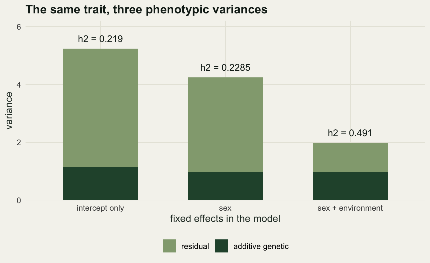
There is no correct answer to which of the three is the heritability. There is a correct answer to which one answers a given question. If you want to predict the response of the population mean to selection acting on the trait as the animals actually experience it, the denominator should contain the variance that selection sees, which usually means keeping the environmental variation in it. If you want a heritability that is comparable to a laboratory estimate for the same trait, you want the covariate out of the denominator, because the laboratory removed that variation by design rather than by regression.
What is not defensible is reporting the number without the model. A heritability of 0.491 and a heritability of 0.219 are the same population here, and the only way a reader can tell which one they are looking at is if the fixed effect structure is written down next to it. This is the single most common reason two published heritabilities for the same trait are not comparable, and it costs one sentence in the methods to prevent.
There is a second habit that helps, and it costs almost as little. Report the variance components themselves, not only the ratio. If the additive variance, the residual variance and the sample size are in the table, a later reader can rebuild any denominator they like, including the one their own study used. A ratio alone cannot be converted into anything. This is also the form in which the estimate is most useful to a meta-analysis, because variances can be pooled sensibly and ratios of variances cannot.
Check three: heritability is not a constant of the trait
The second check moved the denominator by changing the model. The third moves it by changing the environment, which is worse, because it means the heritability of a trait is a statement about a population in a place at a time and not a property of the trait.
The demonstration is direct. Hold the additive variance fixed at 1 and raise the residual variance from 0.5 to 8, then estimate the heritability each time, forty replicates per level. Alongside the heritability, compute the mean standardised additive variance, \(I_A = \sigma^2_a / \bar{z}^2\), which is Houle’s evolvability: the expected proportional change in the mean under a unit strength of selection.
set.seed(20260730)
ve_grid <- c(0.5, 1, 2, 4, 8)
n_rep_c <- 40
sweep_tab <- data.frame(v_e_set = ve_grid, true_h2 = 1 / (1 + ve_grid),
                        h2 = NA_real_, i_a = NA_real_, v_a = NA_real_)
for (i in seq_along(ve_grid)) {
  hh <- numeric(n_rep_c)
  ii <- numeric(n_rep_c)
  vv <- numeric(n_rep_c)
  for (r in seq_len(n_rep_c)) {
    y <- 10 + breeding_values(1) + rnorm(n_ind, 0, sqrt(ve_grid[i]))
    fit <- reml(y, matrix(1, n_ind, 1), ev_true)
    hh[r] <- fit$h2
    ii[r] <- fit$va / mean(y)^2
    vv[r] <- fit$va
  }
  sweep_tab$h2[i] <- mean(hh)
  sweep_tab$i_a[i] <- mean(ii)
  sweep_tab$v_a[i] <- mean(vv)
}
print(round(sweep_tab, 4))
v_e_set true_h2 h2 i_a v_a
1 0.5 0.6667 0.6338 0.0094 0.9383
2 1.0 0.5000 0.4958 0.0099 0.9988
3 2.0 0.3333 0.3152 0.0097 0.9766
4 4.0 0.2000 0.2144 0.0107 1.0848
5 8.0 0.1111 0.1246 0.0111 1.1138print(round(c(replicates_per_level = n_rep_c,
true_i_a = 1 / 10^2,
h2_fall = sweep_tab$h2[1] - sweep_tab$h2[5],
i_a_change = sweep_tab$i_a[5] - sweep_tab$i_a[1],
h2_fold_change = sweep_tab$h2[1] / sweep_tab$h2[5]), 4))replicates_per_level true_i_a h2_fall
40.0000 0.0100 0.5092
i_a_change h2_fold_change
0.0017 5.0874 The heritability falls from 0.6338 to 0.1246 across the sweep, a drop of 0.5092, with the additive variance held at 1 throughout and estimated at between 0.9383 and 1.1138. Move the same animals to a noisier environment and their heritability drops by a factor of 5.0874 with no genetic change of any kind. The evolvability moves from 0.0094 to 0.0111, which is a change of 0.0017 on a quantity whose true value is 0.01.
This is the sense in which a heritability is not a property of a trait. The same genotypes, the same additive variance, the same everything except the amount of environmental noise, and the number that gets reported changes by fivefold. Two studies of the same species can report heritabilities that differ by that much without either of them being wrong, and without there being any genetic difference between the populations at all. A garden with irrigation and a hillside without one are enough.
That small upward drift in the evolvability is not nothing, and it is the fourth check announcing itself early. At the noisiest level the true heritability is only 0.1111, and the additive variance estimate there is 1.1138, slightly above the true 1. That is the boundary at zero pushing the average up, which is the subject of the last section. Note also that the estimated heritability at that level, 0.1246, is above its true value of 0.1111 for the same reason, while at the least noisy level the estimate 0.6338 sits below its true value of 0.6667. Nothing about the sweep is a clean unbiased ladder, and the sign of the deviation flips with the size of the true value.
The consequence is that heritability and evolvability rank traits differently, and the difference is not subtle. Four traits are simulated on the same pedigree, chosen to look like the ones a passerine study actually measures: a skeletal trait with a large mean and small variance, a wing measurement, a clutch size, and an annual count of fledglings. The residual variances are set so that the skeletal traits are the heritable ones, which is what real data say. Mean standardisation is scale free in the sense that switching from millimetres to centimetres leaves the evolvability alone, since it divides the additive variance and the squared mean by the same factor. What it is not free of is the origin: the trait needs a meaningful zero, which is why this works for lengths and counts and does not work for something like a date.
set.seed(20260802)
traits <- data.frame(
  trait = c("tarsus length", "wing length", "clutch size", "annual fledglings"),
  trait_mean = c(20, 60, 5, 4),
  v_a_set = c(0.45, 9, 0.30, 0.5),
  v_e_set = c(0.45, 13.5, 1.20, 4.5))
n_rep_t <- 60
traits$h2 <- NA_real_
traits$i_a <- NA_real_
for (i in seq_len(nrow(traits))) {
  hh <- numeric(n_rep_t)
  ii <- numeric(n_rep_t)
  for (r in seq_len(n_rep_t)) {
    y <- traits$trait_mean[i] + breeding_values(traits$v_a_set[i]) +
      rnorm(n_ind, 0, sqrt(traits$v_e_set[i]))
    fit <- reml(y, matrix(1, n_ind, 1), ev_true)
    hh[r] <- fit$h2
    ii[r] <- fit$va / mean(y)^2
  }
  traits$h2[i] <- mean(hh)
  traits$i_a[i] <- mean(ii)
}
traits$rank_by_h2 <- rank(-traits$h2)
traits$rank_by_i_a <- rank(-traits$i_a)
trait_out <- traits[, c("trait", "h2", "i_a", "rank_by_h2", "rank_by_i_a")]
trait_out$h2 <- round(trait_out$h2, 4)
trait_out$i_a <- round(trait_out$i_a, 4)
print(trait_out)
trait h2 i_a rank_by_h2 rank_by_i_a
1 tarsus length 0.5045 0.0011 1 4
2 wing length 0.4021 0.0025 2 3
3 clutch size 0.1885 0.0112 3 2
4 annual fledglings 0.1024 0.0324 4 1print(round(c(replicates_per_trait = n_rep_t,
rank_correlation = cor(traits$rank_by_h2, traits$rank_by_i_a),
evolvability_ratio = traits$i_a[4] / traits$i_a[1],
h2_ratio = traits$h2[1] / traits$h2[4]), 4))replicates_per_trait rank_correlation evolvability_ratio
60.0000 -1.0000 28.3060
h2_ratio
4.9261 The two rankings are exactly reversed: the rank correlation is -1. Tarsus length has the highest heritability, 0.5045, and the lowest evolvability, 0.0011. Annual fledglings has the lowest heritability, 0.1024, and the highest evolvability, 0.0324, which is 28.306 times larger. On the heritability scale tarsus length beats annual fledglings by a factor of 4.9261; on the evolvability scale the order is the other way round and the gap is several times wider.
slope_dat <- rbind(
  data.frame(trait = traits$trait, x = 1, y = traits$rank_by_h2),
  data.frame(trait = traits$trait, x = 2, y = traits$rank_by_i_a))
lab_left <- data.frame(trait = traits$trait, x = 0.94, y = traits$rank_by_h2,
                       txt = paste0(traits$trait, "  ",
                                    sprintf("%.4f", traits$h2)))
lab_right <- data.frame(trait = traits$trait, x = 2.06, y = traits$rank_by_i_a,
                        txt = paste0(sprintf("%.4f", traits$i_a), "  ",
                                     traits$trait))

ggplot(slope_dat, aes(x, y, colour = trait, group = trait)) +
  geom_line(linewidth = 1) +
  geom_point(size = 2.6) +
  geom_text(data = lab_left, aes(x, y, label = txt), inherit.aes = FALSE,
            hjust = 1, size = 3.5, colour = te_pal$ink) +
  geom_text(data = lab_right, aes(x, y, label = txt), inherit.aes = FALSE,
            hjust = 0, size = 3.5, colour = te_pal$ink) +
  scale_colour_manual(values = c("tarsus length" = te_pal$forest,
                                 "wing length" = te_pal$green,
                                 "clutch size" = te_pal$gold,
                                 "annual fledglings" = te_pal$clay)) +
  scale_x_continuous(breaks = c(1, 2), limits = c(0.35, 2.72),
                     labels = c("ranked by heritability", "ranked by evolvability")) +
  scale_y_reverse(breaks = 1:4) +
  labs(x = NULL, y = "rank", title = "Two summaries, opposite orders") +
  theme_te() +
  theme(legend.position = "none", panel.grid.major.x = element_blank())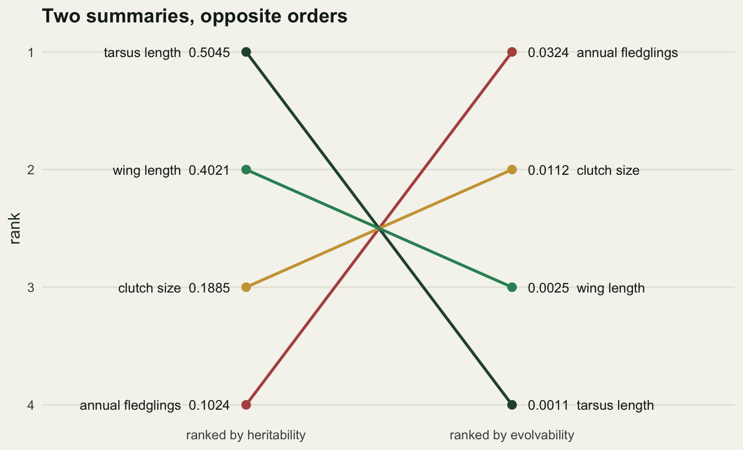
The simulation did not discover that pattern; the input variances were chosen to imitate one that real data show, in which life history traits have low heritabilities because their residual variance is large rather than because they lack additive variance. What the simulation does show is the consequence. Scaled by the mean rather than by the phenotypic variance, those same traits turn out to be the most variable things in the data set. A trait can have a heritability of 0.1024 and still be the trait that responds fastest to selection on a proportional scale.
Which summary you should report depends on the question, and the two questions are genuinely different. Heritability answers “what fraction of the differences I can see are heritable”, which is what you want when predicting the response to a selection differential measured in trait units. Evolvability answers “how fast can the mean move, proportionally”, which is what you want when comparing traits with different units or different scales. The mistake is to report one and interpret it as the other, and the ranking above is what that mistake costs.
Check four: the sampling distribution and the boundary
The last check is about the number you attach to the estimate rather than the estimate itself. A variance cannot be negative, so a heritability cannot be either, and the fitter above enforces that by searching an interval whose lower end is exactly zero. When the true heritability is small the unconstrained maximum is often negative, and the constrained one is then exactly zero. A sample of estimates piles up on the boundary.
Three hundred replicates with a true heritability of 0.05 on this pedigree, which is a small but entirely publishable value for a behavioural trait in a wild population.
set.seed(20260731)
n_rep_d <- 300
true_small <- 0.05
h2_small <- numeric(n_rep_d)
lrt_small <- numeric(n_rep_d)
for (r in seq_len(n_rep_d)) {
  y <- 10 + breeding_values(true_small) + rnorm(n_ind, 0, sqrt(1 - true_small))
  fit <- reml(y, matrix(1, n_ind, 1), ev_true)
  h2_small[r] <- fit$h2
  lrt_small[r] <- fit$lrt
}
print(round(c(replicates = n_rep_d,
              true_h2 = true_small,
              proportion_exactly_zero = mean(h2_small == 0),
              mean_estimate = mean(h2_small),
              upward_bias = mean(h2_small) - true_small,
              median_estimate = median(h2_small),
              mean_of_nonzero = mean(h2_small[h2_small > 0]),
              upper_decile = as.vector(quantile(h2_small, 0.9))), 4))
replicates true_h2 proportion_exactly_zero
300.0000 0.0500 0.2700
mean_estimate upward_bias median_estimate
0.0649 0.0149 0.0477
mean_of_nonzero upper_decile
0.0890 0.1558 Exactly zero came back from 0.27 of the 300 replicates. The mean of the estimates is 0.0649 against a true value of 0.05, so the average is biased upward by 0.0149, while the median is 0.0477 and sits close to the truth. The average of the replicates that did not hit the boundary is 0.089, nearly twice the true value.
Both halves of that matter. The full distribution has an upward biased mean because the boundary truncates the low side and nothing truncates the high side. The published literature contains a selected version of this distribution, because a study that estimates exactly zero writes a different paper from one that estimates 0.1558, the upper decile here. A boundary and a publication filter together make small positive heritabilities.
Now the test. The obvious thing to do with a small estimate is to test it against zero with a likelihood ratio and one degree of freedom. The null hypothesis puts the parameter on the boundary of the space, so the standard asymptotics do not apply; the correct reference is a fifty fifty mixture of a chi-squared with one degree of freedom and a point mass at zero. The measurement below simulates the null directly: three hundred data sets with no additive variance at all.
set.seed(20260803)
lrt_null <- numeric(n_rep_d)
for (r in seq_len(n_rep_d)) {
  y <- 10 + rnorm(n_ind, 0, 1)
  lrt_null[r] <- reml(y, matrix(1, n_ind, 1), ev_true)$lrt
}
probs <- c(0.90, 0.95, 0.99)
q_tab <- data.frame(
  quantile = probs,
  empirical = as.vector(quantile(lrt_null, probs)),
  chisq_1_df = qchisq(probs, 1),
  mixture = qchisq(1 - 2 * (1 - probs), 1))
print(round(q_tab, 4))
quantile empirical chisq_1_df mixture
1 0.90 1.3998 2.7055 1.6424
2 0.95 2.0274 3.8415 2.7055
3 0.99 4.0786 6.6349 5.4119print(round(c(replicates = n_rep_d,
proportion_lrt_exactly_zero = mean(lrt_null == 0),
error_rate_naive_test = mean(lrt_null > qchisq(0.95, 1)),
error_rate_mixture_test = mean(lrt_null > qchisq(0.90, 1))), 4)) replicates proportion_lrt_exactly_zero
300.0000 0.5267
error_rate_naive_test error_rate_mixture_test
0.0167 0.0400 Under the null, 0.5267 of the test statistics are exactly zero, which is the point mass the mixture predicts and the chi-squared with one degree of freedom does not have at all. The empirical 95th percentile of the null distribution is 2.0274. The chi-squared reference puts it at 3.8415 and the mixture puts it at 2.7055. The empirical value sits below both, closer to the mixture.
grid_x <- seq(0, 8, length.out = 241)
cdf_dat <- rbind(
  data.frame(x = grid_x, y = sapply(grid_x, function(z) mean(lrt_null <= z)),
             series = "empirical null (300 replicates)"),
  data.frame(x = grid_x, y = pchisq(grid_x, 1),
             series = "chi-squared, 1 df"),
  data.frame(x = grid_x, y = 0.5 + 0.5 * pchisq(grid_x, 1),
             series = "50:50 mixture"))
cdf_dat$series <- factor(cdf_dat$series,
                         levels = c("empirical null (300 replicates)",
                                    "50:50 mixture", "chi-squared, 1 df"))

ggplot(cdf_dat, aes(x, y, colour = series)) +
  geom_line(linewidth = 1) +
  scale_colour_manual(values = c(te_pal$clay, te_pal$forest, te_pal$gold), name = NULL) +
  scale_y_continuous(limits = c(0, 1.02), expand = c(0, 0)) +
  labs(x = "restricted likelihood ratio statistic", y = "cumulative probability",
       title = "The null is not a chi-squared with one degree of freedom") +
  guides(colour = guide_legend(nrow = 1)) +
  theme_te()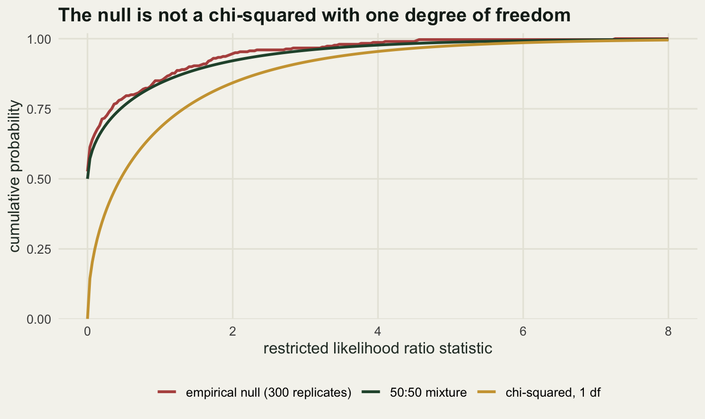
The practical consequence is the error rate. Testing at the nominal five per cent with the chi-squared reference, which is what happens whenever somebody compares two nested models and reads a p-value off one degree of freedom, rejects on 0.0167 of these null data sets. The mixture reference, which puts the five per cent critical value at 2.7055, rejects on 0.04.
The direction of that error surprises people, and it is the third measured result here that runs against the reflex. A boundary problem sounds like it should make the test too eager. It does the opposite: the naive test is conservative, spending 0.0167 of the 0.05 it is nominally allowed, because it is using a reference distribution that is too spread out. So the error is not that you find heritabilities that are not there. It is that you miss ones that are, and the size of that loss is measurable from the replicates already in hand: the same test statistics computed at a true heritability of 0.05.
print(round(c(replicates = n_rep_d,
              true_h2 = true_small,
              power_naive_reference = mean(lrt_small > qchisq(0.95, 1)),
              power_mixture_reference = mean(lrt_small > qchisq(0.90, 1)),
              detections_gained = sum(lrt_small > qchisq(0.90, 1)) -
                sum(lrt_small > qchisq(0.95, 1))), 4))
replicates true_h2 power_naive_reference
300.0000 0.0500 0.1333
power_mixture_reference detections_gained
0.1767 13.0000 At a true heritability of 0.05 the naive test rejects in 0.1333 of replicates and the mixture test in 0.1767: a difference of 13 detections out of 300. Neither is a well powered test, which is its own lesson about a pedigree this size.
The fix costs nothing. Halve the p-value from the one degree of freedom test, or compare the statistic against 2.7055 instead of 3.8415 for a five per cent test. Report the estimate with a confidence interval that is allowed to touch zero rather than a p-value alone, and say which reference you used.
What to take away
Four checks, four things that could change what you report. A recorded pedigree with wrong fathers attenuates the estimate, but by the errors-in-variables factor rather than by the fraction of wrong links: at a sire error rate of 0.4 the estimate kept 0.7693 of its value where the arithmetic in your head said 0.6. The fixed effect structure moved the same heritability from 0.219 to 0.491. Raising environmental noise alone moved it from 0.6338 to 0.1246 while the evolvability barely moved, and the two summaries ranked four traits in exactly opposite orders. At a true heritability of 0.05, 0.27 of replicates landed exactly on zero and the naive likelihood ratio test rejected at 0.0167 rather than 0.05.
None of these is a reason to distrust animal models. They are reasons to report the model along with the number: the fixed effects, the pedigree and how the paternities were assigned, the interval rather than the point, and the reference distribution behind any test against zero. A heritability without those four things is not a measurement, it is a decoration.
The honest limit: everything above is one simulated pedigree of 330 individuals with Gaussian traits, correctly specified apart from the thing being checked, with paternity errors drawn at random with respect to breeding value, so the numbers are conditional on that setup and would move with a deeper pedigree, a count trait, or extra-pair sires that are themselves selected for high breeding values. The replicate counts are small on purpose, 32 per error rate and 300 for the boundary work, so third decimal places here are noise; what carries is the direction and the rough size of each effect, and both of those were stable across the seeds tried while writing this.
References
Wilson AJ, Reale D, Clements MN, Morrissey MM, Postma E, Walling CA, Kruuk LEB, Nussey DH 2010 Journal of Animal Ecology 79(1):13-26 (10.1111/j.1365-2656.2009.01639.x)
Kruuk LEB 2004 Philosophical Transactions of the Royal Society B 359(1446):873-890 (10.1098/rstb.2003.1437)
Houle D 1992 Genetics 130(1):195-204 (10.1093/genetics/130.1.195)
Hansen TF, Pelabon C, Houle D 2011 Evolutionary Biology 38(3):258-277 (10.1007/s11692-011-9127-6)
Patterson HD, Thompson R 1971 Biometrika 58(3):545-554 (10.1093/biomet/58.3.545)
Self SG, Liang KY 1987 Journal of the American Statistical Association 82(398):605-610 (10.1080/01621459.1987.10478472)
Lynch M, Walsh B 1998 Genetics and Analysis of Quantitative Traits (ISBN 978-0-87893-481-2)