library(ggplot2)

te_pal <- list(forest = "#275139", green = "#2f8f63", sage = "#93a87f",
               clay = "#b5534e", gold = "#cda23f", line = "#dad9ca",
               ink = "#16241d", paper = "#f5f4ee")

theme_te <- function() {
  theme_minimal(base_size = 12) +
    theme(panel.grid.minor = element_blank(),
          panel.grid.major = element_line(colour = "#e7e6dc"),
          plot.background = element_rect(fill = "#f5f4ee", colour = NA),
          panel.background = element_rect(fill = "#f5f4ee", colour = NA),
          plot.title = element_text(face = "bold", colour = te_pal$ink),
          axis.title = element_text(colour = "#2c3a31"),
          legend.position = "bottom")
}Maternal effects inflate heritability
R
quantitative genetics
heritability
study design
ecology tutorial
A base R simulation of how a shared nest inflates heritability in an animal model, why full sibs alone cannot separate the two, and what cross-fostering buys.
The ringing happens on day fourteen. You open the box, lift out the brood, and work through them one at a time: ring number, tarsus, mass, back in the box before the female gets agitated. Eight chicks from one box, six from the next, and by the end of the week you have several hundred nestlings from sixty boxes in the same beech wood, all measured with the same calipers.
Those eight chicks share their parents. They also share a box, a pair of adults running caterpillars back and forth, a position in the wood, and whatever the weather did during the week they were growing fastest. When you feed the measurements into an animal model and it reports a heritability above one half for tarsus length, the model has assigned all of that shared similarity to the only thing in it that makes relatives resemble each other: the additive genetic variance. The wood, the caterpillars and the female’s provisioning rate have nowhere else to go.
Everyone who fits these models knows this, and the usual response is to add a random effect for the nest. This post measures what that buys you. It simulates pedigrees where full sibs share a nest of known variance, fits both models, and asks how big the inflation is, whether the data can tell the two models apart, and what a design has to look like before the separation means anything. The middle question is the one that matters, and the answer is more brutal than the usual warning suggests.
Everything below is written in base R and ggplot2. The relationship matrix, the restricted likelihood and the optimiser are all a few dozen lines. The animal model post explains where the numerator relationship matrix and the restricted likelihood come from; here the same machinery is rebuilt compactly so this post stands on its own.
Two models, one pedigree
The first model says that the phenotype of individual \(i\) is a mean plus a breeding value plus noise, \(y_i = \mu + a_i + e_i\), with the vector of breeding values distributed as \(N(0, A\sigma^2_a)\) where \(A\) is the numerator relationship matrix. The second model adds a nest term, \(y_i = \mu + a_i + n_{j(i)} + e_i\), with the nest effects independent and identically distributed with variance \(\sigma^2_n\). In matrix form the two phenotypic covariance structures are
\[V_1 = A\sigma^2_a + I\sigma^2_e, \qquad V_2 = A\sigma^2_a + ZZ'\sigma^2_n + I\sigma^2_e\]
where \(ZZ'\) is one for every pair reared in the same nest and zero otherwise.
The numerator relationship matrix comes from the tabular method: process the pedigree with parents before offspring, and fill each new row from the rows of the parents.
amat <- function(sire, dam) {
  n <- length(sire)
  A <- matrix(0, n, n)
  for (i in seq_len(n)) {
    s <- sire[i]; d <- dam[i]
    if (i > 1L) {
      j <- seq_len(i - 1L)
      v <- 0.5 * ((if (s > 0L) A[j, s] else 0) + (if (d > 0L) A[j, d] else 0))
      A[i, j] <- v; A[j, i] <- v
    }
    A[i, i] <- 1 + if (s > 0L && d > 0L) 0.5 * A[s, d] else 0
  }
  A
}

## one sire, one dam, two full sib offspring
print(amat(c(0, 0, 1, 1), c(0, 0, 2, 2)))
[,1] [,2] [,3] [,4]
[1,] 1.0 0.0 0.5 0.5
[2,] 0.0 1.0 0.5 0.5
[3,] 0.5 0.5 1.0 0.5
[4,] 0.5 0.5 0.5 1.0The bottom right corner of that small matrix is the whole problem in miniature. Two full sibs have a relationship of 0.5, so the animal model expects them to covary by half the additive variance. If they also share a nest, they covary by half the additive variance plus the whole nest variance, and the first model has only one dial to turn.
The restricted likelihood is the standard one for a single fixed effect, an intercept. Written at absolute variances it is the function below. Fitting is faster if the residual variance is profiled out, which leaves two variance ratios to optimise over, so both forms are here: reml_ll for looking at the surface, reml_prof for fitting.
reml_ll <- function(y, Ao, Zn, s) {
  n <- length(y)
  V <- s[1] * Ao + s[3] * diag(n)
  if (!is.null(Zn)) V <- V + s[2] * Zn
  ch <- chol(V)
  Viy <- backsolve(ch, backsolve(ch, y, transpose = TRUE))
  Vi1 <- backsolve(ch, backsolve(ch, rep(1, n), transpose = TRUE))
  s11 <- sum(Vi1)
  yPy <- sum(y * Viy) - sum(y * Vi1)^2 / s11
  -0.5 * (2 * sum(log(diag(ch))) + log(s11) + yPy)
}

reml_prof <- function(y, Ao, Zn, r) {
  n <- length(y)
  H <- diag(n) + r[1] * Ao
  if (!is.null(Zn)) H <- H + r[2] * Zn
  ch <- chol(H)
  Hiy <- backsolve(ch, backsolve(ch, y, transpose = TRUE))
  Hi1 <- backsolve(ch, backsolve(ch, rep(1, n), transpose = TRUE))
  s11 <- sum(Hi1)
  yPy <- sum(y * Hiy) - sum(y * Hi1)^2 / s11
  list(ll = -0.5 * ((n - 1) * log(yPy / (n - 1)) + 2 * sum(log(diag(ch))) +
                      log(s11) + (n - 1)),
       se2 = yPy / (n - 1))
}

fit_a <- function(y, Ao) {
  o <- optimize(function(lr) -reml_prof(y, Ao, NULL, c(exp(lr), 0))$ll,
                c(-10, 4), tol = 1e-4)
  ra <- exp(o$minimum); p <- reml_prof(y, Ao, NULL, c(ra, 0))
  c(sa2 = ra * p$se2, sn2 = 0, se2 = p$se2, h2 = ra / (1 + ra), ll = p$ll)
}

fit_an <- function(y, Ao, Zn, start = c(-1.2, -1.2)) {
  o <- optim(start, function(lr) -reml_prof(y, Ao, Zn, exp(pmax(pmin(lr, 4), -10)))$ll,
             method = "Nelder-Mead", control = list(reltol = 1e-6))
  r <- exp(pmax(pmin(o$par, 4), -10)); p <- reml_prof(y, Ao, Zn, r)
  tot <- (r[1] + r[2] + 1) * p$se2
  c(sa2 = r[1] * p$se2, sn2 = r[2] * p$se2, se2 = p$se2,
    h2 = r[1] * p$se2 / tot, c2 = r[2] * p$se2 / tot, ll = p$ll)
}
Two designs are compared throughout, deliberately the same size. In the first, every dam is mated to her own sire, so the only relatives are full sibs and every full sib group is a nest. In the second, each sire is mated to several dams, so the data also contain paternal half sibs: pairs that share genes but were reared in different boxes.
make_design <- function(n_sire, dams_per_sire, k) {
  n_dam <- n_sire * dams_per_sire
  n_off <- n_dam * k
  n_ped <- n_sire + n_dam + n_off
  sire <- integer(n_ped); dam <- integer(n_ped)
  off <- n_sire + n_dam + seq_len(n_off)
  sire[off] <- rep(rep(seq_len(n_sire), each = dams_per_sire), each = k)
  dam[off] <- rep(n_sire + seq_len(n_dam), each = k)
  A <- amat(sire, dam)
  list(A = A, L = t(chol(A)), Ao = A[off, off], off = off, n_ped = n_ped,
       nest = rep(seq_len(n_dam), each = k), n_off = n_off, n_nest = n_dam)
}

zz_of <- function(nest) outer(nest, nest, "==") * 1

sim_y <- function(d, sa2, sn2, se2, nest = d$nest) {
  a <- as.vector(d$L %*% rnorm(d$n_ped)) * sqrt(sa2)
  a[d$off] + rnorm(max(nest), 0, sqrt(sn2))[nest] + rnorm(d$n_off, 0, sqrt(se2))
}

k_off <- 4L
sib <- make_design(25L, 1L, k_off)
hs <- make_design(5L, 5L, k_off)
Zs <- zz_of(sib$nest); Zh <- zz_of(hs$nest)
sa2_true <- 0.3; h2_true <- 0.3
print(c(offspring = sib$n_off, nests = sib$n_nest, brood_size = k_off,
        sires_sib_design = 25L, sires_halfsib_design = 5L, dams_per_sire = 5L))
offspring nests brood_size
100 25 4
sires_sib_design sires_halfsib_design dams_per_sire
25 5 5 print(round(c(sa2_true = sa2_true, total_variance = 1, h2_true = h2_true), 3)) sa2_true total_variance h2_true
0.3 1.0 0.3 cat("relatedness classes, full sib design\n")relatedness classes, full sib designprint(table(round(sib$Ao[upper.tri(sib$Ao)], 4)))
   0  0.5
4800 150 cat("relatedness classes, half sib design\n")relatedness classes, half sib designprint(table(round(hs$Ao[upper.tri(hs$Ao)], 4)))
   0 0.25  0.5
4000  800  150
Both designs have 100 offspring in 25 nests of 4. The full sib design contains 150 pairs at relatedness 0.5 and 4800 unrelated pairs, with no intermediate class. The half sib design contains the same 150 full sib pairs plus 800 paternal half sib pairs at relatedness 0.25. The true additive variance is 0.3, the total phenotypic variance is held at 1 as the nest variance is varied, so the true heritability is 0.3 in every cell.
What the missing nest term costs
The first experiment walks the true nest variance up a grid and, in each cell, simulates both designs and fits both models. Everything is small on purpose: a hundred replicates per cell, a hundred animals per replicate. The estimator is noisy at that size, which is the point, and the interest is in the mean across replicates rather than in any single fit.
set.seed(41010727)
reps <- 100L; vgrid <- c(0, 0.1, 0.2, 0.3, 0.4)
E1 <- NULL; cell0 <- NULL
for (v in vgrid) {
  se2 <- 1 - sa2_true - v
  m <- matrix(NA_real_, reps, 5)
  for (i in seq_len(reps)) {
    ys <- sim_y(sib, sa2_true, v, se2)
    yh <- sim_y(hs, sa2_true, v, se2)
    m[i, 1] <- fit_a(ys, sib$Ao)["h2"]
    m[i, 2] <- fit_a(yh, hs$Ao)["h2"]
    m[i, 3:5] <- fit_an(yh, hs$Ao, Zh)[c("h2", "c2", "sn2")]
  }
  if (v == 0) cell0 <- m
  E1 <- rbind(E1, data.frame(nest_var = v, sibs_no_nest = mean(m[, 1]),
    hs_no_nest = mean(m[, 2]), hs_with_nest = mean(m[, 3]),
    hs_nest_share = mean(m[, 4]), sd_sibs_no_nest = sd(m[, 1]),
    sd_hs_no_nest = sd(m[, 2]), sd_hs_with_nest = sd(m[, 3])))
}
print(round(E1, 3))
nest_var sibs_no_nest hs_no_nest hs_with_nest hs_nest_share sd_sibs_no_nest
1 0.0 0.301 0.273 0.190 0.046 0.198
2 0.1 0.446 0.539 0.271 0.117 0.209
3 0.2 0.647 0.727 0.256 0.205 0.204
4 0.3 0.848 0.902 0.292 0.289 0.167
5 0.4 0.939 0.975 0.303 0.377 0.102
sd_hs_no_nest sd_hs_with_nest
1 0.226 0.190
2 0.252 0.261
3 0.229 0.266
4 0.152 0.335
5 0.026 0.330print(c(replicates_per_cell = reps))replicates_per_cell
100 print(round(c(
slope_sibs = unname(coef(lm(sibs_no_nest ~ nest_var, E1[1:4, ]))[2]),
slope_halfsib = unname(coef(lm(hs_no_nest ~ nest_var, E1[1:4, ]))[2])), 3)) slope_sibs slope_halfsib
1.843 2.076 Read the first column of that table. With no nest effect at all the model without a nest term recovers the truth: 0.301 against a true 0.3. Push the nest variance to 0.2 and the same model reports 0.647. Push it to 0.3 and it reports 0.848, which is to say that most of the variation in a trait with a heritability of 0.3 is now being called genetic.
The rate is the interesting part. Fitting a straight line to the first four cells gives a slope of 1.843 in the full sib design. The heritability does not rise by the nest variance; it rises by about twice the nest variance. The algebra behind that is short. With unrelated families, all the covariance information in the data is the covariance between full sibs, which is \(0.5\sigma^2_a + \sigma^2_n\). A model with no nest term must reproduce that covariance using \(0.5\sigma^2_a\) alone, so its additive variance has to be \(\sigma^2_a + 2\sigma^2_n\). The shared environment is not just misattributed. It is misattributed and doubled on the way, because the model divides it by the relatedness of the pairs that display it.
Now compare the two designs. The obvious expectation is that half sibs help: they give the model a second, independent view of the additive variance, from pairs that never shared a box. The measurement says otherwise. At a nest variance of 0.2 the full sib design returns 0.647 and the half sib design returns 0.727. The fitted slope is 2.076 with half sibs against 1.843 without them. Adding half sibs did not reduce the bias of the wrong model, and by these numbers it made it slightly worse.
That separates two ideas that get run together: a design that identifies a parameter is not a design that protects you from omitting it. Restricted maximum likelihood fits the covariance structure you handed it, and given a structure with one source of resemblance it reconciles the full sib and half sib covariances as best it can. The full sib pairs carry the inflated covariance, so the compromise still lands high. Half sibs make the correct model estimable and do nothing whatsoever for the incorrect one.
The third column is the model with the nest term on the half sib design. Its mean estimate sits between 0.190 and 0.303 across the whole grid, against a true 0.3, and the estimated nest share tracks the true nest variance from 0.046 up to 0.377. That is what a correctly specified model looks like: not accurate in any one replicate, but pointed at the right place.
lab_mod <- c("full sibs, no nest term", "half sibs, no nest term",
             "half sibs, nest term")
fa <- data.frame(nest_var = rep(E1$nest_var, 3),
                 h2 = c(E1$sibs_no_nest, E1$hs_no_nest, E1$hs_with_nest),
                 model = factor(rep(lab_mod, each = nrow(E1)), levels = lab_mod))
ggplot(fa, aes(nest_var, h2, colour = model, shape = model)) +
  geom_hline(yintercept = h2_true, linetype = "dashed",
             colour = te_pal$sage, linewidth = 0.7) +
  geom_line(linewidth = 0.8) +
  geom_point(size = 2.6) +
  scale_colour_manual(values = c(te_pal$clay, te_pal$gold, te_pal$forest)) +
  scale_shape_manual(values = c(16, 17, 15)) +
  scale_y_continuous(limits = c(0, 1)) +
  labs(x = "true nest variance", y = "mean estimated heritability",
       colour = NULL, shape = NULL) + theme_te()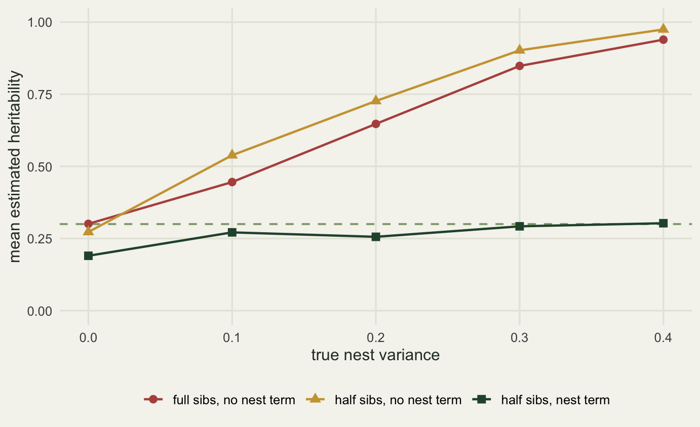
Why full sibs alone cannot answer this
The natural next move is to fit the model with the nest term to the full sib data and be done. This does not work, and the reason is not statistical delicacy. It is arithmetic.
Take the full sib design and write out the phenotypic covariance matrix. Within a brood of size \(k\) it is \(I(0.5\sigma^2_a + \sigma^2_e) + J(0.5\sigma^2_a + \sigma^2_n)\), where \(J\) is a block of ones, and between broods it is zero. The likelihood sees the data only through those two quantities. Call them \(p = 0.5\sigma^2_a + \sigma^2_e\) and \(q = 0.5\sigma^2_a + \sigma^2_n\). Two numbers, three parameters. Any triple with the same \(p\) and the same \(q\) gives byte for byte the same likelihood.
set.seed(20260727)
truth_demo <- data.frame(additive = sa2_true, nest = 0.2, residual = 0.5)
print(truth_demo)
additive nest residual
1 0.3 0.2 0.5y_sib <- sim_y(sib, truth_demo$additive, truth_demo$nest, truth_demo$residual)
y_hs <- sim_y(hs, truth_demo$additive, truth_demo$nest, truth_demo$residual)
t1 <- c(0.20, 0.15, 0.60)
t2 <- c(0.50, 0.00, 0.45)
print(data.frame(triple = c("first", "second"),
additive = c(t1[1], t2[1]), nest = c(t1[2], t2[2]),
residual = c(t1[3], t2[3]),
ll = round(c(reml_ll(y_sib, sib$Ao, Zs, t1),
reml_ll(y_sib, sib$Ao, Zs, t2)), 5))) triple additive nest residual ll
1 first 0.2 0.15 0.60 -36.52392
2 second 0.5 0.00 0.45 -36.52392starts <- rbind(c(-3, 0.5), c(-1.2, -1.2), c(0.5, -3))
ms_sib <- t(apply(starts, 1, function(s) fit_an(y_sib, sib$Ao, Zs, s)))
ms_hs <- t(apply(starts, 1, function(s) fit_an(y_hs, hs$Ao, Zh, s)))
cat("three starting values, full sib data\n")three starting values, full sib dataprint(round(ms_sib, 4)) sa2 sn2 se2 h2 c2 ll
[1,] 0.0409 0.4675 0.4321 0.0435 0.4971 -32.5992
[2,] 0.1528 0.4122 0.3760 0.1624 0.4381 -32.5992
[3,] 0.8730 0.0519 0.0160 0.9279 0.0552 -32.5992cat("three starting values, half sib data\n")three starting values, half sib dataprint(round(ms_hs, 4)) sa2 sn2 se2 h2 c2 ll
[1,] 0.1138 0.1861 0.5889 0.1280 0.2094 -40.9432
[2,] 0.1170 0.1857 0.5868 0.1316 0.2088 -40.9432
[3,] 0.1145 0.1862 0.5883 0.1288 0.2095 -40.9432The first triple puts an additive variance of 0.2 with a nest variance of 0.15; the second puts 0.5 with no nest variance at all. One says the trait is barely heritable and the box does the work, the other says the box does nothing. Both report a restricted log likelihood of -36.52392, and the difference between them is zero to every decimal place printed. Not small. Zero.
The three optimiser runs make the same point in the form you will actually meet it. On the full sib data the three starting values return heritabilities of 0.0435, 0.1624 and 0.9279, and all three report a log likelihood of -32.5992. The fitting routine did not fail and it did not warn. It converged three times, to three different answers, each of which fits the data exactly as well as the others. On the half sib data the same three starts return 0.1280, 0.1316 and 0.1288, all at a log likelihood of -40.9432. Same code, same optimiser, different design.
The surface itself is worth drawing. Because the flat direction keeps \(\sigma^2_a + \sigma^2_n + \sigma^2_e\) constant, a slice at the fitted total variance contains the whole of it, so a two dimensional picture loses nothing.
vp_sib <- sum(ms_sib[2, 1:3]); vp_hs <- sum(ms_hs[2, 1:3])

## profile the nest variance out, one additive variance at a time
prof_sa2 <- function(y, Ao, Zn, vp, a) {
  -optimize(function(nn) -reml_ll(y, Ao, Zn, c(a, nn, vp - a - nn)),
            c(1e-4, vp - a - 0.02), tol = 1e-4)$objective
}
ag <- seq(0.02, 0.84, by = 0.02)
P1 <- sapply(ag, function(a) prof_sa2(y_sib, sib$Ao, Zs, vp_sib, a))
P2 <- sapply(ag, function(a) prof_sa2(y_hs, hs$Ao, Zh, vp_hs, a))
flat <- function(p) range(ag[p > max(p) - 0.1])
print(data.frame(design = c("full sibs", "half sibs"),
                 total_variance = round(c(vp_sib, vp_hs), 3),
                 flat_from = c(flat(P1)[1], flat(P2)[1]),
                 flat_to = c(flat(P1)[2], flat(P2)[2]),
                 searched = paste(min(ag), "to", max(ag))))
design total_variance flat_from flat_to searched
1 full sibs 0.941 0.02 0.84 0.02 to 0.84
2 half sibs 0.890 0.02 0.26 0.02 to 0.84## the surface itself, on the slice through the fitted total variance
gsa <- seq(0.01, 0.7, length.out = 51)
gsn <- seq(0.01, 0.5, length.out = 51)
surf <- function(y, Ao, Zn, vp) {
z <- outer(gsa, gsn, Vectorize(function(a, nn) {
e <- vp - a - nn
if (e <= 0.02) return(-500)
reml_ll(y, Ao, Zn, c(a, nn, e))
}))
z - max(z)
}
S1 <- surf(y_sib, sib$Ao, Zs, vp_sib); S2 <- surf(y_hs, hs$Ao, Zh, vp_hs)Profiling the nest variance out, one additive variance at a time, gives the width of the near maximal region. In the full sib design the additive variance can be set anywhere from 0.02 to 0.84 without the restricted log likelihood dropping by even a tenth of a unit, and those are the two ends of the range that was searched: the profile is flat from one end to the other and the search, not the data, decided where to stop. In the half sib design the near maximal region for the additive variance reaches up to 0.26. The lower end is again the bottom of the searched grid, and that same grid caps how far up the profile could be followed at all. At an additive variance of 0.01, the left edge of the surface drawn below, the profile is still only 0.078 below its maximum.
gr <- expand.grid(sa2 = gsa, sn2 = gsn)
sur <- rbind(data.frame(gr, ll = as.vector(S1), design = "full sibs only"),
             data.frame(gr, ll = as.vector(S2), design = "with paternal half sibs"))
sur$ll <- pmax(sur$ll, -3)
sur$vp <- rep(c(vp_sib, vp_hs), each = nrow(gr))
no_room <- sur[sur$vp - sur$sa2 - sur$sn2 <= 0.02, ]
ggplot(sur, aes(sa2, sn2)) +
  geom_raster(aes(fill = ll)) +
  geom_contour(aes(z = ll), breaks = c(-0.1, -0.5, -1, -2),
               colour = "#f5f4ee", linewidth = 0.3) +
  geom_raster(data = no_room, fill = "#b9b7a8") +
  annotate("point", x = sa2_true, y = 0.2, colour = te_pal$paper,
           shape = 4, size = 4.2, stroke = 3) +
  annotate("point", x = sa2_true, y = 0.2, colour = te_pal$clay,
           shape = 4, size = 3.4, stroke = 1.6) +
  facet_wrap(~ design) +
  scale_fill_gradient(low = "#12291d", high = te_pal$gold,
                      name = "log likelihood from maximum") +
  labs(x = "additive variance", y = "nest variance") + theme_te() +
  theme(panel.grid.major = element_blank(),
        legend.key.width = unit(1.6, "cm"))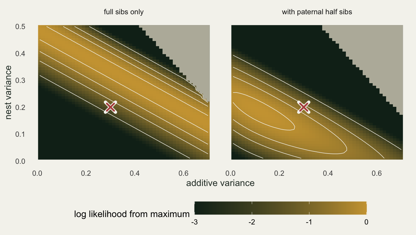
What sixty starting values tell you
If one optimiser run cannot be trusted here, sixty runs from sixty starting values can at least map what it was choosing between, at a cost of a few hundredths of a second per fit.
set.seed(60060727)
n_start <- 60L
st <- cbind(runif(n_start, -4, 1), runif(n_start, -4, 1))
multi <- function(y, Ao, Zn) t(apply(st, 1, function(s) fit_an(y, Ao, Zn, s)))
Q1 <- multi(y_sib, sib$Ao, Zs)
Q2 <- multi(y_hs, hs$Ao, Zh)

print(c(starting_values = n_start))
starting_values
60 print(data.frame(
design = c("full sibs", "half sibs"),
h2_min = round(c(min(Q1[, "h2"]), min(Q2[, "h2"])), 4),
h2_max = round(c(max(Q1[, "h2"]), max(Q2[, "h2"])), 4),
sa2_min = round(c(min(Q1[, "sa2"]), min(Q2[, "sa2"])), 4),
sa2_max = round(c(max(Q1[, "sa2"]), max(Q2[, "sa2"])), 4),
ll_range = round(c(diff(range(Q1[, "ll"])), diff(range(Q2[, "ll"]))), 4),
slope = round(c(unname(coef(lm(Q1[, "sn2"] ~ Q1[, "sa2"]))[2]),
unname(coef(lm(Q2[, "sn2"] ~ Q2[, "sa2"]))[2])), 4))) design h2_min h2_max sa2_min sa2_max ll_range slope
1 full sibs 0.0174 0.9285 0.0164 0.8732 0.0000 -0.5000
2 half sibs 0.1266 0.1907 0.1124 0.1712 0.0143 -0.2891On the full sib data the sixty runs return heritabilities from 0.0174 to 0.9285, and the largest difference in restricted log likelihood among them is zero to four decimal places. Every one of those answers is a maximum likelihood estimate. They lie on a line whose slope is -0.5000, which is the algebra reappearing: holding \(q = 0.5\sigma^2_a + \sigma^2_n\) fixed means every unit of additive variance you add buys exactly half a unit of nest variance removed.
On the half sib data the sixty runs land between 0.1266 and 0.1907, with a log likelihood range of 0.0143. That spread is not a ridge. It is the optimiser stopping at its tolerance, and the likelihood values differ, so the poorer starts are visibly worse fits and could be discarded on that basis. On the full sib data there is nothing to discard.
fc <- rbind(data.frame(sa2 = Q1[, "sa2"], sn2 = Q1[, "sn2"],
                       design = "full sibs only"),
            data.frame(sa2 = Q2[, "sa2"], sn2 = Q2[, "sn2"],
                       design = "with paternal half sibs"))
ggplot(fc, aes(sa2, sn2)) +
  geom_point(colour = te_pal$forest, size = 2.1, alpha = 0.75) +
  annotate("point", x = sa2_true, y = 0.2, colour = te_pal$clay,
           shape = 4, size = 3.4, stroke = 1.2) +
  facet_wrap(~ design) +
  labs(x = "estimated additive variance", y = "estimated nest variance") +
  theme_te()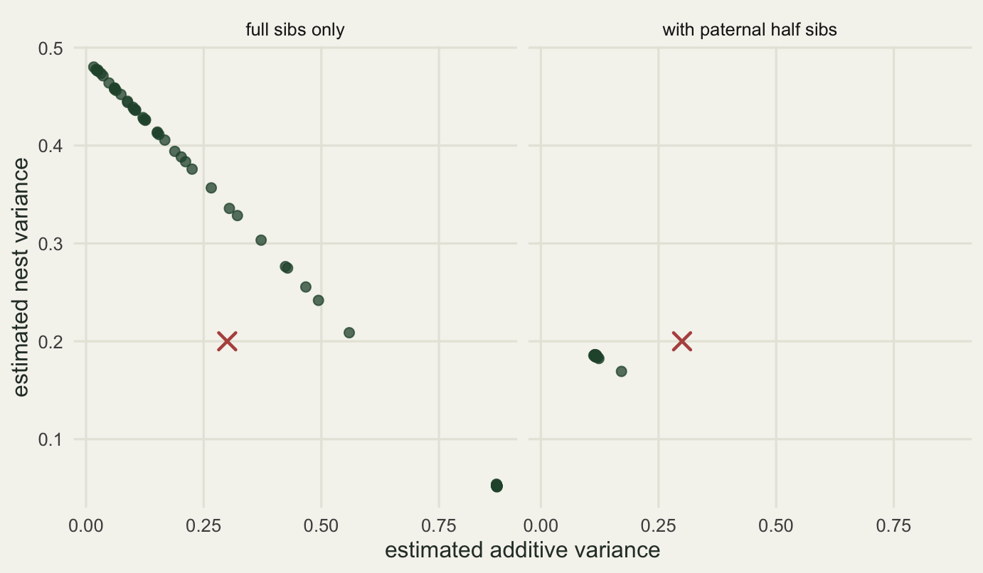
There is a trap hiding in all this, and it is the reason the problem survives in published work. Run the full sib fit once per replicate from the same starting value, as everybody does, and look at how much the answer moves across replicates.
set.seed(20260728)
reps2 <- 120L
R1 <- matrix(NA_real_, reps2, 3); R2 <- matrix(NA_real_, reps2, 3)
fixed_h2 <- numeric(reps2); dll <- numeric(reps2)
for (i in seq_len(reps2)) {
  ys <- sim_y(sib, sa2_true, 0.2, 0.5)
  yh <- sim_y(hs, sa2_true, 0.2, 0.5)
  a1 <- fit_an(ys, sib$Ao, Zs, runif(2, -3, 0))
  a0 <- fit_an(ys, sib$Ao, Zs)
  a2 <- fit_an(yh, hs$Ao, Zh, runif(2, -3, 0))
  b1 <- fit_a(ys, sib$Ao)
  R1[i, ] <- a1[c("sa2", "sn2", "h2")]; R2[i, ] <- a2[c("sa2", "sn2", "h2")]
  fixed_h2[i] <- a0["h2"]; dll[i] <- a0["ll"] - b1["ll"]
}
print(c(replicates = reps2))
replicates
120 print(round(c(mean_h2_sibs_fixed_start = mean(fixed_h2),
sd_h2_sibs_fixed_start = sd(fixed_h2),
h2_implied_by_the_start = exp(-1.2) / (1 + 2 * exp(-1.2)),
mean_h2_halfsib = mean(R2[, 3]), sd_h2_halfsib = sd(R2[, 3]),
corr_sibs = cor(R1[, 1], R1[, 2]),
corr_halfsib = cor(R2[, 1], R2[, 2])), 3))mean_h2_sibs_fixed_start sd_h2_sibs_fixed_start h2_implied_by_the_start
0.197 0.034 0.188
mean_h2_halfsib sd_h2_halfsib corr_sibs
0.280 0.289 -0.502
corr_halfsib
-0.534 print(round(c(mean_ll_gain = mean(dll), max_ll_gain = max(dll),
frac_gain_above_001 = mean(dll > 0.001),
frac_lrt_significant = mean(2 * dll > 2.706)), 4)) mean_ll_gain max_ll_gain frac_gain_above_001
0.0216 1.2852 0.1000
frac_lrt_significant
0.0000 Across 120 replicates, the full sib heritability estimate from a fixed starting value has a standard deviation of 0.034. The half sib estimate, from data of identical size and a correctly specified model, has a standard deviation of 0.289, which is more than eight times larger. On the usual reading of those two numbers, the full sib design is the precise one. It is the opposite. The full sib estimate barely moves because it is barely a function of the data at all: its mean across replicates is 0.197, and the heritability implied by the starting value handed to the optimiser is 0.188. The routine is returning its own starting value with a small data dependent correction, and stability across replicates is the symptom, not the reassurance.
One diagnostic that gets suggested for this, the correlation between the two variance estimates across replicates, does not work either. It is -0.502 in the full sib design and -0.534 in the half sib design. The two components trade off against each other in both, because they always do; the correlation cannot see the difference between a trade off that the data resolve and one that they do not. Refitting from scattered starts and comparing likelihoods does see it, and costs a few seconds.
Now the piece that has to be said plainly, because it is the honest limit of every analysis in this post. If the design is full sibs with no fostering, the data cannot choose between the two models. The nest model gained 0.0216 log likelihood units on average over the model without a nest term, its largest gain in 120 replicates was 1.2852, and the number of replicates where a likelihood ratio test would have called the nest term significant was zero. Not one. The nest variance in this simulation was two thirds of the additive variance, and the likelihood never noticed.
The likelihood is not merely underpowered here but blind, for the reason from the last section: the model without a nest term is a point on the ridge, so it reaches the same maximum, provided it can get there with a non negative residual variance. That fails only when the full sib correlation exceeds one half.
set.seed(20260729)
reps3 <- 100L
big <- data.frame(additive = sa2_true, nest = 0.45, residual = 0.25)
d2 <- numeric(reps3)
for (i in seq_len(reps3)) {
  ys <- sim_y(sib, big$additive, big$nest, big$residual)
  d2[i] <- fit_an(ys, sib$Ao, Zs)["ll"] - fit_a(ys, sib$Ao)["ll"]
}
print(c(replicates = reps3))
replicates
100 print(data.frame(big,
full_sib_correlation = 0.5 * big$additive + big$nest,
mean_ll_gain = round(mean(d2), 3),
frac_lrt_significant = mean(2 * d2 > 2.706))) additive nest residual full_sib_correlation mean_ll_gain frac_lrt_significant
1 0.3 0.45 0.25 0.6 1.201 0.33With a nest variance of 0.45 the true full sib correlation is 0.6, above the half that pure additive inheritance can produce. Now the mean likelihood gain is 1.201 and a likelihood ratio test rejects the smaller model in a fraction 0.33 of the 100 replicates. A shared environment large enough to break the physical ceiling on sib similarity is detectable from sib data alone, and only just. Anything smaller is invisible.
Cross-fostering buys the separation
The design fix that does not require extra sires is to move chicks. Swap a fraction of the brood between boxes soon after hatching and the nest stops being a synonym for the family: some boxes now hold chicks from several broods, and some sibships are spread across several boxes. The model can then attribute similarity to whichever grouping carries it.
foster <- function(nest, f) {
  n <- length(nest); m <- round(f * n)
  if (m < 2) return(nest)
  idx <- sample.int(n, m)
  nest[idx] <- nest[sample(idx)]
  nest
}

set.seed(30070727)
fr <- c(0, 0.1, 0.25, 0.5, 0.75, 1); repsf <- 120L
E3 <- NULL
for (f in fr) {
  m <- matrix(NA_real_, repsf, 2)
  for (i in seq_len(repsf)) {
    nn <- foster(sib$nest, f)
    ys <- sim_y(sib, sa2_true, 0.2, 0.5, nest = nn)
    m[i, ] <- fit_an(ys, sib$Ao, zz_of(nn))[c("h2", "c2")]
  }
  E3 <- rbind(E3, data.frame(fostered = f, mean_h2 = mean(m[, 1]),
    sd_h2 = sd(m[, 1]), sd_nest_share = sd(m[, 2]), corr = cor(m[, 1], m[, 2])))
}
print(round(E3, 3))
fostered mean_h2 sd_h2 sd_nest_share corr
1 0.00 0.201 0.033 0.118 -0.682
2 0.10 0.302 0.295 0.156 -0.708
3 0.25 0.308 0.227 0.112 -0.546
4 0.50 0.323 0.194 0.108 -0.343
5 0.75 0.293 0.178 0.102 -0.197
6 1.00 0.295 0.185 0.098 -0.239print(c(replicates_per_fraction = repsf))replicates_per_fraction
120 print(round(c(gain_realised_at_half =
(E3$sd_h2[2] - E3$sd_h2[4]) / (E3$sd_h2[2] - E3$sd_h2[5])), 3))gain_realised_at_half
0.865 Start at the bottom of the table and work up. With every chick fostered, the heritability estimate has a mean of 0.295 against a true 0.3 and a standard deviation of 0.185. Fostering a tenth of the chicks already makes the model estimable: the mean is 0.302, close enough to the truth, but the standard deviation is 0.295, larger than at full fostering. Half fostered brings it to 0.194, which is 0.865 of the gain available between a tenth and three quarters. Beyond a half the curve is flat, and the difference between 0.194 at half and 0.178 at three quarters is inside the Monte Carlo noise of 120 replicates.
The correlation between the two estimates falls steadily as fostering rises, from -0.708 at a tenth fostered to -0.197 at three quarters: the trade off loosening as more chicks end up in foreign boxes.
The top row is the one to read carefully, and it is the trap from the previous section in table form. With nothing fostered, the standard deviation of the heritability estimate is 0.033, by far the smallest number in that column, and the mean is 0.201. A design that cannot identify the parameter at all produces the most stable estimate in the experiment, sitting on the value the optimiser was started from. Precision measured as replicate to replicate variability is not evidence of anything until you know the parameter is identified.
fd <- rbind(data.frame(f = E3$fostered, s = E3$sd_h2, quantity = "heritability"),
            data.frame(f = E3$fostered, s = E3$sd_nest_share,
                       quantity = "nest share of variance"))
ggplot(fd, aes(f, s, colour = quantity, shape = quantity)) +
  geom_line(data = fd[fd$f > 0, ], linewidth = 0.8) +
  geom_point(size = 2.6) +
  annotate("text", x = 0.02, y = 0.055, hjust = 0, size = 3.4,
           colour = te_pal$ink, label = "no fostering: not identified") +
  scale_colour_manual(values = c(te_pal$forest, te_pal$gold)) +
  scale_shape_manual(values = c(16, 17)) +
  scale_y_continuous(limits = c(0, 0.34)) +
  labs(x = "fraction of chicks fostered", colour = NULL, shape = NULL,
       y = "standard deviation across replicates") + theme_te()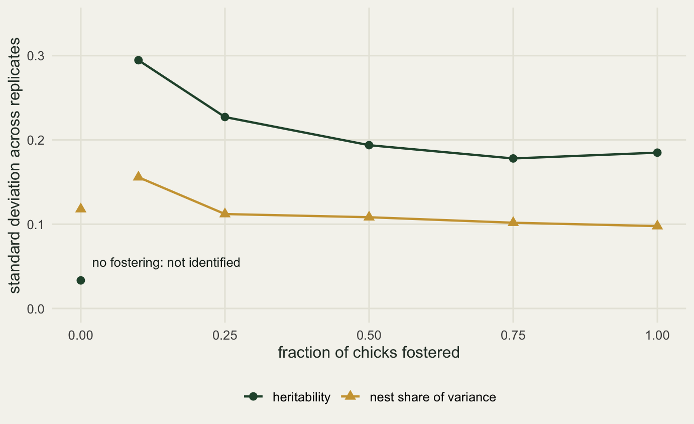
A maternal effect is not a nest effect
Up to here the shared environment has been a box: an effect drawn once per nest, independent of everything else, exactly matching the term the model fits. Real maternal effects are not like that. If a female’s condition determines how much she provisions, the offspring phenotype depends on the mother’s phenotype, and her phenotype contains her breeding value. The shared effect is then correlated with the thing the model is trying to estimate, and it passes down the pedigree rather than being sprinkled over nests.
The simulation below builds a pedigree with a generation of grandsires, so the dams fall into groups of paternal half sibs, unrelated between groups. Every dam has her own phenotype \(z_d = a_d + e_d\), and each of her offspring gets \(y = a + m z_d + e\). The parameter \(m\) is the strength of the maternal path. Nests are still full sib broods, and there are still paternal half sibs among the offspring, so the additive variance is identified.
n_gsire <- 5L; dams_per_gsire <- 5L; n_msire <- 5L
n_mdam <- n_gsire * dams_per_gsire; n_moff <- n_mdam * k_off
gsire <- seq_len(n_gsire); msire <- n_gsire + seq_len(n_msire)
mdam <- n_gsire + n_msire + seq_len(n_mdam)
moff <- n_gsire + n_msire + n_mdam + seq_len(n_moff)
n_mped <- n_gsire + n_msire + n_mdam + n_moff
sire_m <- integer(n_mped); dam_m <- integer(n_mped)
sire_m[mdam] <- rep(gsire, each = dams_per_gsire)
dam_of_off <- rep(as.vector(sapply(seq_len(n_msire), function(s)
  mdam[(seq_len(n_gsire) - 1L) * dams_per_gsire + s])), each = k_off)
sire_m[moff] <- rep(msire, each = n_gsire * k_off); dam_m[moff] <- dam_of_off

Am <- amat(sire_m, dam_m); Lm <- t(chol(Am))
Amo <- Am[moff, moff]
Zm <- zz_of(rep(seq_len(n_mdam), each = k_off))
print(c(offspring = n_moff, nests = n_mdam, grandsires = n_gsire,
        sires = n_msire))
offspring nests grandsires sires
100 25 5 5 cat("relatedness classes among offspring\n")relatedness classes among offspringprint(table(round(Amo[upper.tri(Amo)], 4)))
     0 0.0625   0.25    0.5
  3200    800    800    150
The offspring now fall into three classes of relative: full sibs at 0.5, paternal half sibs at 0.25 whose dams are unrelated, and pairs at 0.0625 whose dams are half sibs. That last class is the one that will do the talking.
Under the maternal model the covariance between two offspring is not \(A_{ij}\sigma^2_a\) plus a nest term. It is
\[C_{ij} = A_{ij}\sigma^2_a + m\sigma^2_a(A_{i,d_j} + A_{j,d_i}) + m^2 \mathrm{Cov}(z_{d_i}, z_{d_j})\]
where \(A_{i,d_j}\) is the relationship between offspring \(i\) and the dam of offspring \(j\). Every one of those terms is computable from the pedigree, so the prediction can be checked against the simulation directly.
se2_m <- 0.7
Aod <- Am[moff, dam_of_off]; same_dam <- outer(dam_of_off, dam_of_off, "==") * 1
cov_pred <- function(m) sa2_true * Amo + m * sa2_true * (Aod + t(Aod)) +
  m^2 * (sa2_true * Am[dam_of_off, dam_of_off] + se2_m * same_dam)

sim_mat <- function(m) {
  a <- as.vector(Lm %*% rnorm(n_mped)) * sqrt(sa2_true)
  zd <- a[mdam] + rnorm(n_mdam, 0, sqrt(se2_m))
  a[moff] + m * zd[match(dam_of_off, mdam)] + rnorm(n_moff, 0, sqrt(se2_m))
}

cls <- round(Amo, 4); ut <- upper.tri(cls)
lv <- sort(unique(cls[ut]))
msk <- lapply(lv, function(l) which(ut & cls == l))
set.seed(40040727)
reps_cov <- 600L; repsm <- 100L
MAT <- NULL; COV <- NULL
for (mm in c(0.4, -0.25)) {
  cv <- matrix(NA_real_, reps_cov, length(lv))
  for (i in seq_len(reps_cov)) {
    y <- sim_mat(mm); cp <- outer(y, y)
    for (j in seq_along(lv)) cv[i, j] <- mean(cp[msk[[j]]])
  }
  cpm <- cov_pred(mm)
  COV <- rbind(COV, data.frame(m = mm, relatedness = lv,
    additive_only = lv * sa2_true,
    with_maternal = sapply(msk, function(w) mean(cpm[w])),
    observed = colMeans(cv)))
  res <- matrix(NA_real_, repsm, 6)
  for (i in seq_len(repsm)) {
    y <- sim_mat(mm)
    res[i, ] <- c(fit_an(y, Amo, Zm)[c("sa2", "sn2", "h2", "c2")],
                  fit_a(y, Amo)["h2"], mean(y^2))
  }
  vp <- sa2_true + mm^2 * (sa2_true + se2_m) + mm * sa2_true + se2_m
  MAT <- rbind(MAT, data.frame(m = mm, phenotypic_var = vp,
    mean_square = mean(res[, 6]), true_h2 = sa2_true / vp,
    sa2_hat = mean(res[, 1]), sn2_hat = mean(res[, 2]),
    h2_with_nest = mean(res[, 3]), h2_no_nest = mean(res[, 5]),
    frac_nest_at_zero = mean(res[, 2] < 0.001)))
}
print(round(COV, 4))
m relatedness additive_only with_maternal observed
1 0.40 0.0000 0.0000 0.0000 0.0005
2 0.40 0.0625 0.0187 0.0608 0.0577
3 0.40 0.2500 0.0750 0.0750 0.0765
4 0.40 0.5000 0.1500 0.4300 0.4216
5 -0.25 0.0000 0.0000 0.0000 0.0012
6 -0.25 0.0625 0.0187 0.0047 0.0064
7 -0.25 0.2500 0.0750 0.0750 0.0733
8 -0.25 0.5000 0.1500 0.1375 0.1314print(round(MAT, 3)) m phenotypic_var mean_square true_h2 sa2_hat sn2_hat h2_with_nest
1 0.40 1.280 1.295 0.234 0.362 0.233 0.270
2 -0.25 0.987 1.001 0.304 0.178 0.037 0.177
h2_no_nest frac_nest_at_zero
1 0.681 0.21
2 0.240 0.55print(c(replicates_for_covariances = reps_cov, replicates_for_fits = repsm))replicates_for_covariances replicates_for_fits
600 100 The covariance table is the argument. Take the positive maternal effect, \(m = 0.4\). Full sibs are predicted to covary by 0.4300 against 0.1500 from genes alone, and they are observed at 0.4216. That part a nest term can absorb. Look one row up. Pairs at relatedness 0.0625, reared in different nests by different mothers, are predicted to covary by 0.0608 where genes alone predict 0.0187, and they are observed at 0.0577. Their similarity is three times what their relatedness would produce, and it happens in different boxes, tended by different mothers, with no shared environment of any kind. The maternal effect went down the pedigree because the dams are relatives.
Paternal half sibs, whose dams are unrelated, sit at 0.0765 against a genetic prediction of 0.0750. They are the only class the maternal effect does not touch, and they are outnumbered by the classes it does. The whole structure checks out against the algebra: the predicted phenotypic variance is 1.280 and the simulated mean square is 1.295.
So the fitted model is pulled two ways. With the nest term in place it returns a heritability of 0.270 against a true value of 0.234, an additive variance of 0.362 against a true 0.3. The nest term did its job on the full sibs, and the model still overstates the heritability, because the excess covariance between the offspring of related dams has nowhere to go except the additive term. Without a nest term the same data give 0.681.
The second row of the table is the case nobody expects. Set \(m = -0.25\), a compensatory maternal effect where large females produce slightly smaller offspring for their genes. The shared component induced within a nest is then \(m^2(\sigma^2_a + \sigma^2_e) + m\sigma^2_a\), and with these values that is negative: full sibs are observed to covary at 0.1314 where their genes alone predict 0.1500. Sibs are less alike than half the additive variance says they should be. A variance component cannot be negative, so the nest term is pinned at zero in more than half the replicates, a fraction 0.55, and the model absorbs the deficit the only way it can, by shrinking the additive variance to 0.178. The heritability comes out at 0.177 against a true 0.304, too low. Adding the nest term made this case worse, not better: without it the same data give 0.240.
A shared nest can only ever inflate a heritability estimate. A maternal effect can push it either way, and the direction depends on the sign of a coefficient that no amount of nest fitting will reveal.
The price of a nest term you do not need
If the nest term is insurance, what is the premium. The first cell of the bias grid answers it: true nest variance zero, half sib design so that both models are estimable, both fitted to the same simulated data sets.
print(round(c(mean_no_nest = mean(cell0[, 2]), mean_with_nest = mean(cell0[, 3]),
              sd_no_nest = sd(cell0[, 2]), sd_with_nest = sd(cell0[, 3]),
              rmse_no_nest = sqrt(mean((cell0[, 2] - h2_true)^2)),
              rmse_with_nest = sqrt(mean((cell0[, 3] - h2_true)^2)),
              frac_nest_at_zero = mean(cell0[, 5] < 0.001)), 3))
mean_no_nest mean_with_nest sd_no_nest sd_with_nest
0.273 0.190 0.226 0.190
rmse_no_nest rmse_with_nest frac_nest_at_zero
0.227 0.219 0.580 The expectation is that the extra parameter costs precision. It does not. The standard deviation of the heritability estimate is 0.226 without the nest term and 0.190 with it, so the model with the extra parameter is the less variable of the two. The reason is in the last number: a fraction 0.580 of replicates put the nest variance at zero, where restricted maximum likelihood keeps it because the estimate is not allowed to go negative. In most replicates the larger model quietly collapses into the smaller one.
The premium is paid somewhere else. The mean estimate is 0.273 without the nest term and 0.190 with it, against a true 0.3. Fitting a nest term that the data do not need pulled the average heritability down. That is the boundary constraint working in one direction only: in the replicates where sampling noise makes sibs look a little more alike than they are, the nest term takes the excess away from the additive variance, and in the replicates where they look less alike, it cannot give anything back. Root mean squared error ends up almost unchanged, 0.227 against 0.219, so the insurance is close to free in total error while being distinctly not free in the number you would put in a table.
What to take away
The order of the findings matters more than any single number. Omitting a shared nest inflates heritability at roughly twice the rate of the nest variance itself, 1.843 per unit here, because the model has to reproduce a full sib covariance using a relatedness of one half. Adding paternal half sibs does not fix that: the wrong model stayed just as wrong, with a slope of 2.076. Half sibs and cross-fostering are what make the right model estimable, and a tenth of the brood fostered is enough to make it estimable while a half is enough to make it reasonably precise.
The honest limit is this: with full sibs and no fostering, nothing in the phenotypes can tell you whether the resemblance is genes or the box, and the model you fit is a decision you made rather than a conclusion you reached. The two models fit the same data equally well, gaining 0.0216 log likelihood units on average and never once reaching significance in 120 replicates, and sixty optimiser starts on one data set returned heritabilities from 0.0174 to 0.9285 at a log likelihood range of 0.0000. No amount of care with the fitting software changes that, because the information is not in the data.
Two habits follow. Refit every variance component model from several scattered starting values and compare the likelihoods rather than the estimates: a design problem shows up as identical likelihoods at different answers, and takes seconds to find. And treat a suspiciously stable estimate as a question, because in the one design here where nothing was identified the estimate was the most stable in the whole post, at a standard deviation of 0.033, and that stability belonged to the optimiser rather than to the birds.
The maternal simulation adds a caution to all of it. A nest term handles an effect shared within a brood and independent between broods. A maternal effect running through the mother’s own phenotype is neither: it travels down the pedigree, so it inflates the additive variance even when a nest term is fitted, and if it is compensatory it deflates the additive variance instead. Separating the two needs dams measured for the same trait, or a design that separates what a mother gives from what she does.
References
Wilson AJ, Reale D, Clements MN, Morrissey MM, Postma E, Walling CA, Kruuk LEB, Nussey DH 2010 Journal of Animal Ecology 79(1):13-26 (10.1111/j.1365-2656.2009.01639.x)
Kruuk LEB 2004 Philosophical Transactions of the Royal Society B 359(1446):873-890 (10.1098/rstb.2003.1437)
Willham RL 1972 Journal of Animal Science 35(6):1288-1293 (10.2527/jas1972.3561288x)
Hadfield JD 2010 Journal of Statistical Software 33(2):1-22 (10.18637/jss.v033.i02)
Lynch M, Walsh B 1998 Genetics and Analysis of Quantitative Traits (ISBN 978-0-87893-481-2)
Falconer DS, Mackay TFC 1996 Introduction to Quantitative Genetics, 4th edition (ISBN 978-0-582-24302-6)