library(ggplot2)
library(patchwork)

te_paper  <- "#f5f4ee"
te_ink    <- "#16241d"
te_body   <- "#2c3a31"
te_forest <- "#275139"
te_rust   <- "#b5534e"
te_gold   <- "#c9b458"
te_line   <- "#dad9ca"

theme_datasheet <- function() {
  theme_minimal(base_size = 12) +
    theme(plot.background  = element_rect(fill = te_paper, colour = NA),
          panel.background = element_rect(fill = te_paper, colour = NA),
          panel.grid.major = element_line(colour = te_line, linewidth = 0.3),
          panel.grid.minor = element_blank(),
          text             = element_text(colour = te_body),
          plot.title       = element_text(colour = te_ink, face = "bold"),
          plot.subtitle    = element_text(colour = te_body),
          axis.text        = element_text(colour = te_body))
}Qst against Fst: is the trait under selection?
R
quantitative genetics
population genetics
simulation
ecology tutorial
Simulate the neutral drift null of Qst in R, measure how often it beats Fst by chance, and see why a one-sided Qst against Fst comparison is not a test.
Six populations of a stream fish, one drainage, a common garden in the basement. Twenty five males per population, each crossed to eight females, one offspring measured per cross: twelve hundred fish reared at the same temperature and fed the same ration, so that whatever divergence remains in body depth is genetic. A panel of markers on the same populations returns an Fst of one tenth. The trait comes out a shade more differentiated than that, and the discussion section writes itself: quantitative divergence exceeds neutral divergence, therefore divergent selection.
That inference rests on a real theorem. For a purely additive trait diverging by drift alone, the Qst formed from the expected variance components is exactly Fst, an equivalence Spitze put to work on Daphnia and which Merila and Crnokrak used to assemble the first large comparison across studies. It is a ratio of expectations, not the expectation of a ratio, and the distance between those two is most of what this post measures.
What a study has is not an expectation. It has one realisation of the drift process in a handful of populations, filtered through a breeding design that estimates two variance components with error. This post measures the operating characteristic of the decision rule that the discussion section actually used: given neutral data, how often does the estimate of Qst come out above Fst? That rate is the false-positive rate of the rule, and it is measured here as a function of the number of populations, the size of the breeding design, and Fst itself.
The neighbouring tutorials cover the pieces. The marker side of the comparison, including how noisy a single locus is and why a negative estimate is information rather than an error, is in the F-statistics post; the machinery for estimating additive genetic variance from relatives is in the animal model post, and how precision depends on the shape of a pedigree is in the pedigree post. Nothing here re-teaches variance components. The axis this post varies is the number of populations, and the object it measures is a decision.
The neutral expectation is a derivation, not a convention
Take a trait controlled by many unlinked additive loci with equal effects. An ancestral population sits at frequency p at every locus. Descendant populations drift independently, which under the standard model leaves each population’s frequency distributed around p with variance Fst * p * (1 - p); the beta distribution with that variance is the usual generator, and it is the same one the F-statistics tutorial uses for marker data.
Write the allelic effect at each locus as a, so a genotype carrying zero, one or two copies has genotypic value zero, a or 2a. Then the population mean at one locus is 2 a p_j, and the variance of that mean across populations is 4 a^2 Fst p (1 - p). Summed over L loci, the among-population component of additive variance is Vb = 4 L a^2 Fst p (1 - p). The additive variance within a population at one locus is 2 a^2 p_j (1 - p_j), whose expectation is 2 a^2 p (1 - p) (1 - Fst), so Vw = 2 L a^2 p (1 - p) (1 - Fst).
Qst for an additive trait is Vb / (Vb + 2 Vw), with the factor of two because drift makes the among-population variance of means twice Fst times the ancestral additive variance, while the within-population component carries no such factor. Substituting gives 4 L a^2 Fst p q / (4 L a^2 Fst p q + 4 L a^2 (1 - Fst) p q), which is Fst. Everything cancels. The number of loci, the allelic effect and the ancestral frequency all leave, which is why the result is quoted as a theorem rather than as a rule of thumb. Lande derived the neutral theory of quantitative variance under structure in this form. The simulation below scales the allelic effect so that the ancestral additive variance is one, and confirms the two components separately.
p_anc  <- 0.5
n_loci <- 100
va_anc <- 1
h2_pop <- 0.3
ve_com <- va_anc * (1 - h2_pop) / h2_pop

draw_pops <- function(n_pop, fst, spread = 1) {
  sh1 <- p_anc * (1 - fst) / fst
  sh2 <- (1 - p_anc) * (1 - fst) / fst
  p_mat <- matrix(rbeta(n_pop * n_loci, sh1, sh2), nrow = n_pop)
  a_eff <- sqrt(va_anc / (2 * n_loci * p_anc * (1 - p_anc)))
  mu_anc <- 2 * a_eff * n_loci * p_anc
  list(mu = mu_anc + spread * (2 * a_eff * rowSums(p_mat) - mu_anc),
       va = 2 * a_eff^2 * rowSums(p_mat * (1 - p_mat)))
}

fst_mark  <- 0.10
alpha_lev <- 0.05
pct_lev   <- 95
n_pop_cal <- 40
n_cal     <- 3000
set.seed(4101)
cal <- t(vapply(seq_len(n_cal), function(i) {
  pp <- draw_pops(n_pop_cal, fst_mark)
  c(vb = var(pp$mu), vw = mean(pp$va))
}, numeric(2)))
vb_cal  <- mean(cal[, "vb"])
vw_cal  <- mean(cal[, "vw"])
qst_cal <- vb_cal / (vb_cal + 2 * vw_cal)
vb_pred <- 2 * fst_mark * va_anc
vw_pred <- (1 - fst_mark) * va_anc
Averaged over 3000 replicate sets of 40 populations, the among-population component is 0.1993 against a predicted 0.2000, and the within-population additive variance is 0.9000 against a predicted 0.9000. The ratio is 0.0997 against an Fst of 0.10. The calibration holds, so anything that follows is a property of estimation and sampling, not of a mis-specified generator.
The spread of population means is not the among-population variance
The design is a paternal half-sib common garden. Each sire is crossed to several dams and one offspring per cross is measured, so offspring sharing a sire are half sibs and nothing else: they do not share a dam, a nest or a maternal environment. The sire variance component is then a quarter of the additive genetic variance, uncontaminated by dominance, by maternal effects or by a common rearing environment, all of which load onto the full-sib covariance. The price is precision. A quarter of the additive variance is a small signal, which is why half-sib designs need many sires.
Nested analysis of variance with populations, sires within populations and offspring within sires gives three mean squares whose expectations are known for a balanced design. Writing sw for the variance among sires within a population, sp for the variance among population means and se for the residual, with f sires per population and n offspring per sire:
E[MS_error] = seE[MS_sire] = se + n swE[MS_pop] = se + n sw + f n sp
Solving downwards recovers the components. The additive genetic variance within populations is 4 sw, and the among-population component sp goes straight into Qst. The naive alternative, which needs no variance components and falls out of a spreadsheet of population means, is to take the observed variance among those means and call it Vb. That quantity is MS_pop / (f n), and its expectation is sp + sw / f + se / (f n). It is the among-population variance plus the sampling variance of the means, and it is biased upwards by an amount the design fixes in advance. The two estimators differ by MS_sire / (f n), which is never negative, so the naive Qst cannot come out below the nested one in any single data set: the direction of every comparison below is algebra, and only the size of the gap is a simulation result.
qst_ratio <- function(vb, vw) {
  vb <- max(vb, 0); vw <- max(vw, 0)
  if (vb <= 0) return(0)
  if (vw <= 0) return(1)
  vb / (vb + 2 * vw)
}
sim_garden <- function(n_pop, n_sire, n_off, fst, spread = 1) {
  pops <- draw_pops(n_pop, fst, spread)
  y <- array(0, dim = c(n_off, n_sire, n_pop))
  for (j in seq_len(n_pop)) {
    sire <- rnorm(n_sire, 0, sqrt(pops$va[j] / 4))
    y[, , j] <- rep(pops$mu[j] + sire, each = n_off) +
      rnorm(n_off * n_sire, 0, sqrt(0.75 * pops$va[j] + ve_com))
  }
  y
}
nested_qst <- function(y) {
  n_off <- dim(y)[1]; n_sire <- dim(y)[2]; n_pop <- dim(y)[3]
  fam_mean <- colMeans(y)
  pop_mean <- colMeans(fam_mean)
  ms_pop  <- n_sire * n_off * sum((pop_mean - mean(pop_mean))^2) / (n_pop - 1)
  ms_sire <- n_off * sum((fam_mean - rep(pop_mean, each = n_sire))^2) /
    (n_pop * (n_sire - 1))
  ms_err <- sum((y - rep(as.vector(fam_mean), each = n_off))^2) /
    (n_pop * n_sire * (n_off - 1))
  v_sire  <- (ms_sire - ms_err) / n_off
  v_among <- (ms_pop - ms_sire) / (n_sire * n_off)
  v_naive <- ms_pop / (n_sire * n_off)
  va_w    <- 4 * v_sire
  c(qst = qst_ratio(v_among, va_w), qst_naive = qst_ratio(v_naive, va_w),
    v_among = v_among, v_naive = v_naive, va_w = va_w)
}
n_pop0 <- 6; n_sire0 <- 25; n_off0 <- 8
set.seed(4102)
garden <- sim_garden(n_pop0, n_sire0, n_off0, fst_mark)
one <- nested_qst(garden)
n_fish <- length(garden)
print(round(one, 4))
qst qst_naive v_among v_naive va_w
0.1022 0.1148 0.1741 0.1983 0.7650 Those 1200 fish were generated with no selection at all. The nested estimate of Qst is 0.1022 and the naive one is 0.1148, and both sit above the marker Fst of 0.10. One neutral data set, of a size most people would call generous, already produces the sentence the discussion section wanted to write. The size of the naive bias is set by the design and not by the biology, so it can be predicted and then measured.
replicate_qst <- function(n_pop, n_sire, n_off, fst, n_rep, spread = 1) {
  t(vapply(seq_len(n_rep),
           function(i) nested_qst(sim_garden(n_pop, n_sire, n_off, fst, spread)),
           numeric(5)))
}
mc_se <- function(p, n) sqrt(p * (1 - p) / n)
design_grid <- list(c(10, 4), c(15, 6), c(25, 8), c(40, 8), c(60, 10))
n_rep_des <- 1500
sw_true <- (1 - fst_mark) * va_anc / 4
se_true <- 0.75 * (1 - fst_mark) * va_anc + ve_com
set.seed(4103)
des <- do.call(rbind, lapply(design_grid, function(dz) {
  r <- replicate_qst(8, dz[1], dz[2], fst_mark, n_rep_des)
  data.frame(sires = dz[1], off = dz[2], per_pop = dz[1] * dz[2],
             vb = mean(r[, "v_among"]), vb_naive = mean(r[, "v_naive"]),
             bias_obs = mean(r[, "v_naive"] - r[, "v_among"]),
             bias_pred = sw_true / dz[1] + se_true / (dz[1] * dz[2]),
             qst = mean(r[, "qst"]), qst_naive = mean(r[, "qst_naive"]),
             fpr = mean(r[, "qst"] > fst_mark),
             fpr_naive = mean(r[, "qst_naive"] > fst_mark),
             zero_frac = mean(r[, "qst"] <= 0), one_frac = mean(r[, "qst"] >= 1))
}))
drop_pts   <- 100 * (des$fpr_naive[1] - des$fpr[1])
drop_mult  <- des$fpr[1] / alpha_lev
print(round(des, 4))
sires off per_pop vb vb_naive bias_obs bias_pred qst qst_naive fpr
1 10 4 40 0.1985 0.2965 0.0980 0.0977 0.2023 0.2468 0.4760
2 15 6 90 0.2019 0.2500 0.0481 0.0484 0.1278 0.1508 0.4800
3 25 8 200 0.2050 0.2290 0.0240 0.0240 0.1074 0.1185 0.4680
4 40 8 320 0.1989 0.2140 0.0151 0.0150 0.1000 0.1069 0.4360
5 60 10 600 0.1980 0.2068 0.0088 0.0088 0.0986 0.1026 0.4307
fpr_naive zero_frac one_frac
1 0.6573 0.0513 0.0847
2 0.5847 0.0180 0.0080
3 0.5413 0.0020 0.0000
4 0.4920 0.0000 0.0000
5 0.4587 0.0000 0.0000The predicted and observed bias agree across the whole sweep: at 40 offspring per population the naive estimator inflates the among-population variance by 0.0980 against a predicted 0.0977, which is 49 per cent of the true component; at 600 offspring per population it is 0.0088 against 0.0088. That agreement is a check on the code and not a finding: bias_pred is the expectation derived above, evaluated at the true components, so the two columns can differ only by Monte Carlo error. Nothing about the inflation is random. It is the sampling variance of a population mean, and a design with more sires and more offspring per sire shrinks it in a way that is known before the first fish is measured.
bias_long <- data.frame(
  per_pop = rep(des$per_pop, 2), qst = c(des$qst, des$qst_naive),
  fpr = c(des$fpr, des$fpr_naive),
  estimator = rep(c("nested ANOVA", "spread of population means"),
                  each = nrow(des)))
est_col <- c(`nested ANOVA` = te_forest, `spread of population means` = te_rust)

p_est <- ggplot(bias_long, aes(per_pop, qst, colour = estimator)) +
  geom_hline(yintercept = fst_mark, colour = te_ink, linetype = "dashed") +
  geom_line(linewidth = 0.9) + geom_point(size = 2.4) +
  scale_x_log10(breaks = des$per_pop) +
  scale_colour_manual(values = est_col, name = NULL) +
  labs(x = "offspring per population (log scale)", y = "mean estimated Qst",
       title = "Mean estimate", subtitle = "dashed: the true Qst of 0.10") +
  theme_datasheet()

p_fpr <- ggplot(bias_long, aes(per_pop, fpr, colour = estimator)) +
  geom_hline(yintercept = alpha_lev, colour = te_ink, linetype = "dashed") +
  geom_line(linewidth = 0.9) + geom_point(size = 2.4) +
  scale_x_log10(breaks = des$per_pop) +
  scale_y_continuous(limits = c(0, 0.75)) +
  scale_colour_manual(values = est_col, name = NULL) +
  labs(x = "offspring per population (log scale)",
       y = "P(estimated Qst > Fst) under drift",
       title = "False positives", subtitle = "dashed: a five per cent test") +
  theme_datasheet()

p_est + p_fpr + plot_layout(guides = "collect") +
  plot_annotation(theme = theme_datasheet() +
                    theme(legend.position = "bottom"))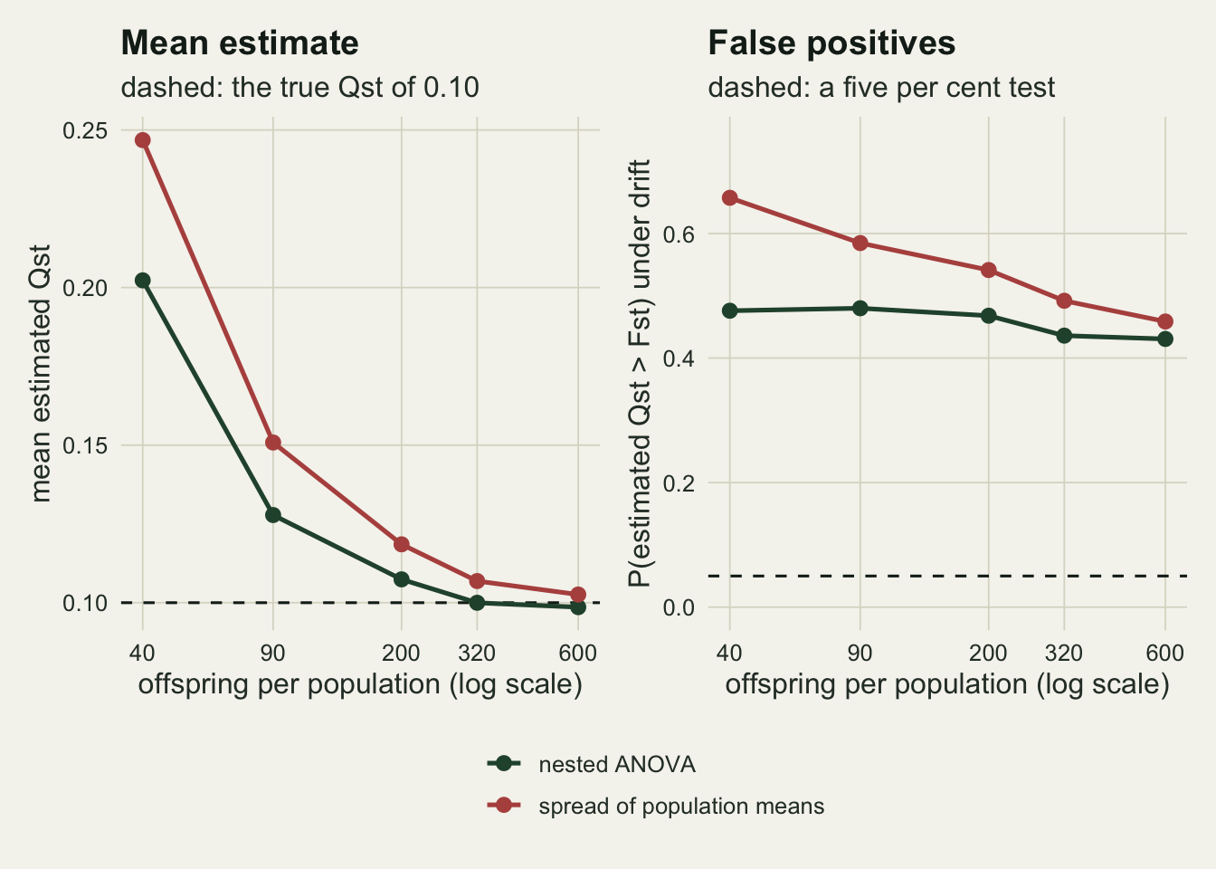
The right panel is the first sign of the real problem. Hold the design fixed at the smallest one and swap the estimator: the rate at which the rule calls selection on neutral data falls from 66 per cent to 48 per cent, a drop of 18 percentage points that still leaves the rule firing 9.5 times as often as its nominal five per cent. Spending on the design does not close the remaining gap either: the largest design in the sweep, 600 offspring per population, still calls selection in 43 per cent of neutral data sets.
Under drift alone, the estimate beats Fst four to five times in ten
That is the point the whole comparison turns on. The theorem fixes the ratio of the expected components at Fst; it does not put the estimator’s own distribution there, and at the marker Fst of 0.10 the grid below has a mean above that value at every number of populations and a median below it. Asking whether an estimate exceeds Fst is therefore asking which side of an off-centre, skewed null one draw happened to fall on. The next simulation runs the full grid: four values of Fst crossed with five numbers of populations, at the intermediate design of 25 sires and 8 offspring each.
d_vec   <- c(3, 5, 8, 16, 32)
fst_vec <- c(0.02, 0.05, 0.10, 0.20)
n_rep   <- 2500
set.seed(4104)
null_raw <- list()
grid_rows <- list()
for (ff in fst_vec) for (dd in d_vec) {
  r <- replicate_qst(dd, n_sire0, n_off0, ff, n_rep)
  if (ff == fst_mark) null_raw[[as.character(dd)]] <- r[, "qst"]
  q95 <- unname(quantile(r[, "qst"], 0.95))
  boot <- replicate(200, quantile(sample(r[, "qst"], n_rep, TRUE), 0.95))
  grid_rows[[sprintf("%g_%d", ff, dd)]] <- data.frame(
    fst = ff, n_pop = dd, mean_qst = mean(r[, "qst"]),
    med_qst = median(r[, "qst"]), mean_naive = mean(r[, "qst_naive"]),
    fpr = mean(r[, "qst"] > ff), fpr_naive = mean(r[, "qst_naive"] > ff),
    fpr25 = mean(r[, "qst"] > 2.5 * ff),
    q95 = q95, mult = q95 / ff, mult_se = sd(boot) / ff)
}
grid_df <- do.call(rbind, grid_rows)
rownames(grid_df) <- NULL
main <- grid_df[grid_df$fst == fst_mark, ]
big_cut <- 2.5 * fst_mark
p_worst  <- 0.5
se_point <- max(mc_se(main$fpr, n_rep))
tail_small <- mean(null_raw[[as.character(d_vec[1])]] > big_cut)
tail_big <- mean(null_raw[[as.character(d_vec[5])]] > big_cut)
fst_at_lo <- range(grid_df$fpr[grid_df$n_pop == d_vec[1]])
fst_at_hi <- range(grid_df$fpr[grid_df$n_pop == d_vec[5]])
spread_lo <- diff(fst_at_lo) / se_point
spread_hi <- diff(fst_at_hi) / se_point
spread_pop <- diff(range(main$fpr)) / se_point
fpr_floor <- min(grid_df$fpr)
floor_mult <- fpr_floor / alpha_lev
print(round(main, 4))
fst n_pop mean_qst med_qst mean_naive fpr fpr_naive fpr25 q95 mult
11 0.1 3 0.1155 0.0703 0.1277 0.3904 0.4352 0.1132 0.3581 3.5812
12 0.1 5 0.1101 0.0879 0.1215 0.4376 0.4928 0.0752 0.2868 2.8685
13 0.1 8 0.1044 0.0937 0.1155 0.4584 0.5332 0.0300 0.2279 2.2786
14 0.1 16 0.1016 0.0950 0.1125 0.4552 0.5664 0.0056 0.1824 1.8240
15 0.1 32 0.1014 0.0986 0.1122 0.4800 0.6316 0.0000 0.1507 1.5067
mult_se
11 0.1162
12 0.0843
13 0.0464
14 0.0304
15 0.0122ecdf_df <- do.call(rbind, lapply(names(null_raw), function(k)
data.frame(qst = null_raw[[k]], pops = factor(k, as.character(d_vec)))))
ggplot(ecdf_df, aes(qst, colour = pops)) +
stat_ecdf(linewidth = 0.8, pad = FALSE) +
geom_vline(xintercept = fst_mark, colour = te_ink, linetype = "dashed") +
coord_cartesian(xlim = c(0, 0.5)) +
scale_colour_manual(values = c(te_rust, te_gold, "#8a9a5b", te_forest,
te_ink), name = "populations") +
labs(x = "estimated Qst under drift alone", y = "cumulative probability",
title = "The neutral null of Qst, by number of populations",
subtitle = "dashed: the marker Fst; the height there is one minus the false-positive rate") +
theme_datasheet() + theme(legend.position = "bottom")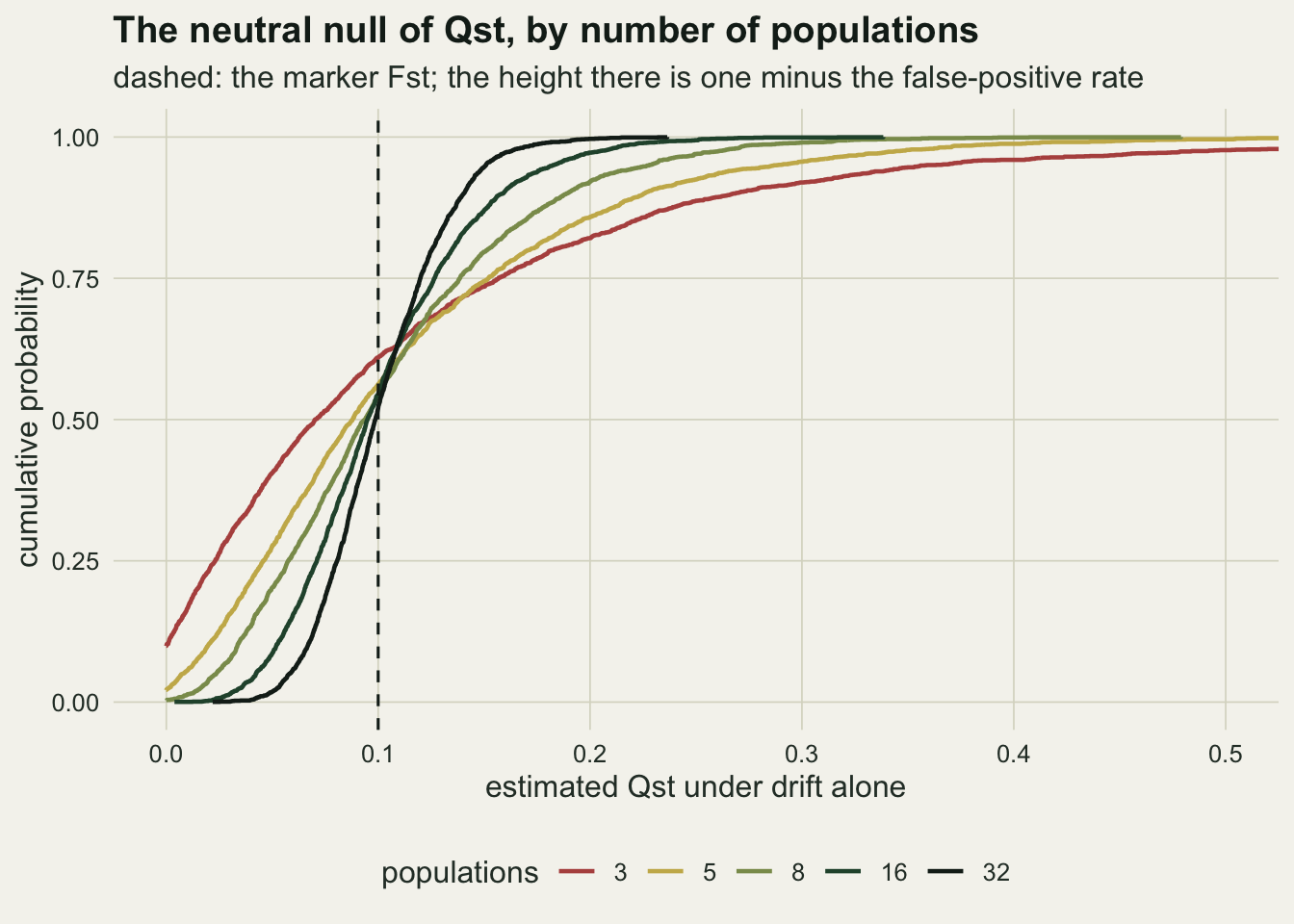
The curves cross the dashed line between 0.52 and 0.61, so the false-positive rate of the rule is 0.39 at 3 populations and 0.48 at 32, with a Monte Carlo standard error of 0.010 on each. The rate is below one half because the null is right-skewed, and the size of that skew is the mean and the median pulling apart: at 3 populations the median estimate is 0.070 while the mean is 0.116, one either side of the Fst of 0.10 the theorem points at. Skew does not rescue the decision. A rule that fires on four or five neutral data sets in ten is not a test at any number of populations.
The number of populations does change the shape of the tail. At 3 populations 11.3 per cent of neutral data sets return an estimate above 0.25, which is two and a half times Fst and would be read as strong evidence; at 32 populations 0 of the 2500 neutral replicates did. Whitlock’s account of what can be inferred from Qst rests on this asymmetry: the distribution is wide and skewed enough that a single estimate, compared with a single number, carries almost no evidential weight on its own.
Adding populations does not repair a biased estimator
Those two rates behave differently as populations are added, and the difference matters more than either one alone.
rule_lab <- c("Qst > Fst, nested ANOVA", "Qst > Fst, spread of means",
              "Qst > 2.5 Fst, nested ANOVA")
rule_col <- setNames(c(te_forest, te_rust, te_gold), rule_lab)
oc_df <- data.frame(n_pop = rep(main$n_pop, 3),
                    rate = c(main$fpr, main$fpr_naive, main$fpr25),
                    rule = factor(rep(rule_lab, each = nrow(main)), rule_lab))
oc_df$se <- mc_se(oc_df$rate, n_rep)

p_oc <- ggplot(oc_df, aes(n_pop, rate, colour = rule)) +
  geom_hline(yintercept = alpha_lev, colour = te_ink, linetype = "dashed") +
  geom_errorbar(aes(ymin = rate - 2 * se, ymax = rate + 2 * se),
                width = 0.06, linewidth = 0.4) +
  geom_line(linewidth = 0.9) + geom_point(size = 2.2) +
  scale_x_log10(breaks = d_vec) +
  scale_colour_manual(values = rule_col, name = NULL) +
  labs(x = "populations (log scale)", y = "false-positive rate under drift",
       title = "Operating characteristic",
       subtitle = "bars: two Monte Carlo standard errors") +
  theme_datasheet() +
  theme(legend.position = "bottom", legend.direction = "vertical")

grid_df$fst_lab <- factor(sprintf("Fst = %.2f", grid_df$fst))
p_mult <- ggplot(grid_df, aes(n_pop, mult, colour = fst_lab)) +
  geom_hline(yintercept = 1, colour = te_ink, linetype = "dashed") +
  geom_line(linewidth = 0.9) + geom_point(size = 2.2) +
  scale_x_log10(breaks = d_vec) +
  scale_colour_manual(values = c(te_rust, te_gold, "#8a9a5b", te_forest),
                      name = NULL) +
  labs(x = "populations (log scale)", y = "critical Qst divided by Fst",
       title = "What a five per cent test needs",
       subtitle = "95th percentile of the drift null") +
  theme_datasheet() +
  theme(legend.position = "bottom", legend.direction = "vertical")

p_oc + p_mult + plot_annotation(theme = theme_datasheet())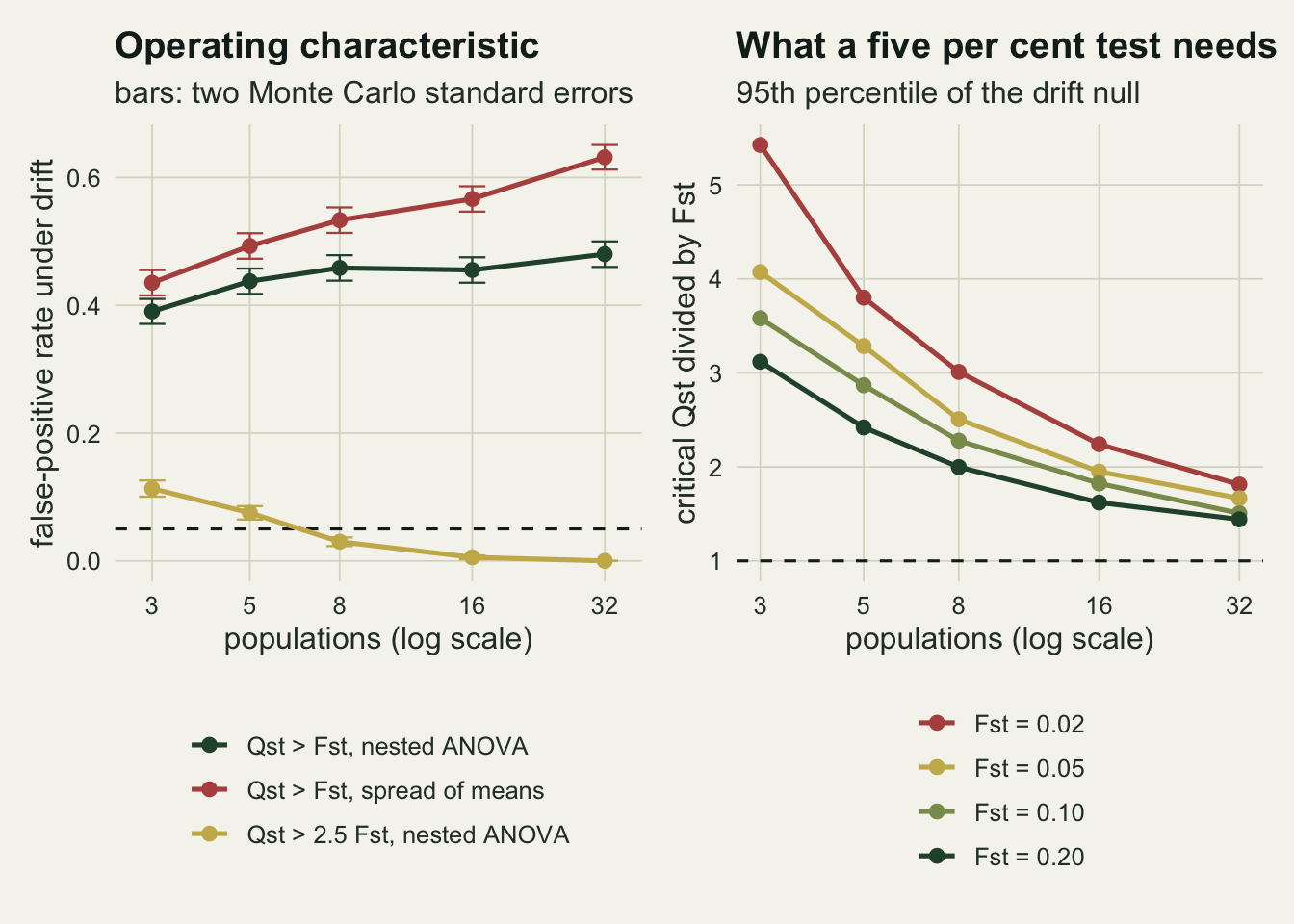
Both point-rule lines in the left panel climb as populations are added, and the difference is where they are heading. The green line is the nested estimator under the point rule, and it rises to 0.48 at 32 populations, approaching one half from below: the estimate is converging on a value that is exactly Fst, so the rule converges on a coin toss. The red line is the same rule applied to the spread of population means, and it goes straight past one half, for a reason worth stating plainly: the bias does not depend on the number of populations, only on the design, so adding populations shrinks the noise around a centre that is in the wrong place. At 3 populations the naive rule fires on 44 per cent of neutral data sets and at 32 populations on 63 per cent. That is the one direction in which this simulation reverses the intuition it started with: more populations make the wrong estimator worse, not better. The reversal is sharper at low differentiation, where the sampling variance of the means is a larger share of a small among-population component.
low <- grid_df[grid_df$fst == fst_vec[1], ]
high <- grid_df[grid_df$fst == fst_vec[4], ]
mult_25 <- (1 - fst_mark) * 2.5 / (1 - 2.5 * fst_mark)
drift_only <- pchisq(mult_25 * (d_vec - 1), d_vec - 1, lower.tail = FALSE)
inflation <- main$fpr25 / drift_only
print(round(data.frame(n_pop = d_vec, measured = main$fpr25,
                       drift_only = drift_only, inflation = inflation), 5))
n_pop measured drift_only inflation
1 3 0.1132 0.04979 2.27368
2 5 0.0752 0.01735 4.33398
3 8 0.0300 0.00377 7.95724
4 16 0.0056 0.00008 73.13316
5 32 0.0000 0.00000 0.00000With an Fst of 0.02 the naive rule fires on 95 per cent of neutral data sets at 32 populations, against 55 per cent when Fst is 0.20. The nested estimator is far less sensitive to Fst than that. Moving along the Fst axis at a fixed number of populations barely shifts its false-positive rate: from 0.390 to 0.417 across the four values of Fst at 3 populations, and from 0.468 to 0.484 at 32, which is 2.8 and 1.6 Monte Carlo standard errors of a single rate. Along the population axis at a single Fst the same rate moves 9.0 standard errors, which is the trend this section opened with. What the grid of 20 combinations shows is not invariance but size: the lowest rate anywhere in it is 0.390, 7.8 times the nominal 0.05, so the failure of the point rule is not a small-sample artefact that a bigger study fixes.
The chunk above also separates the two sources of the wide tail. If the population means were measured without error, the realised among-population variance under drift would be a chi-square variable on one less degree of freedom than the number of populations, and the probability of exceeding two and a half times Fst would be 0.0498 at 3 populations, falling to \(7.66 \times 10^{-5}\) at 16. The measured rates are 0.1132 and 0.0056, so estimation error inflates the rate by a factor of 2.3 at 3 populations and by a factor of 73 at 16. The drift null on its own is only part of the story, and the part that grows in relative importance as populations are added is the breeding design.
The right panel converts all of this into the only number a reader can act on: the multiple of Fst that a Qst estimate has to reach before a genuine one-sided five per cent test would reject. At an Fst of 0.10 it is 3.58 at 3 populations, with a bootstrap standard error of 0.12, and 1.51 at 32. At an Fst of 0.02 it is 5.42 at 3 populations. The threshold depends on Fst as well as on the number of populations, which is why a fixed rule of thumb about how much larger Qst has to be cannot be right everywhere.
A calibrated test exists, and it is weak where it is needed
The repair is not complicated. Simulate the null with the design and the Fst actually in hand, take a high quantile of it, and use that as the critical value. This is the logic Whitlock and Guillaume set out, in a fuller form that also carries the sampling error of Fst itself. What it costs is power, and that cost is measurable.
n_rep_pw <- 1500
crit <- main$q95
set.seed(4105)
pw <- do.call(rbind, lapply(c(3, 5), function(mm) {
  spread <- sqrt((1 - fst_mark) * mm / (1 - mm * fst_mark))
  do.call(rbind, lapply(seq_along(d_vec), function(i) {
    r <- replicate_qst(d_vec[i], n_sire0, n_off0, fst_mark, n_rep_pw, spread)
    data.frame(true_mult = mm, n_pop = d_vec[i], mean_qst = mean(r[, "qst"]),
               pw_point = mean(r[, "qst"] > fst_mark),
               pw_cal = mean(r[, "qst"] > crit[i]))
  }))
}))
print(round(pw, 4))
true_mult n_pop mean_qst pw_point pw_cal
1 3 3 0.2759 0.7707 0.3100
2 3 5 0.2896 0.8800 0.4680
3 3 8 0.2923 0.9513 0.6620
4 3 16 0.2984 0.9947 0.9120
5 3 32 0.2969 1.0000 0.9947
6 5 3 0.4252 0.8967 0.5753
7 5 5 0.4635 0.9680 0.8167
8 5 8 0.4753 0.9960 0.9500
9 5 16 0.4845 1.0000 1.0000
10 5 32 0.4938 1.0000 1.0000Divergent selection is imposed here by scaling each population’s deviation from the ancestral mean, so that the true Qst is three or five times Fst while the within-population architecture is untouched. That is a description of an outcome rather than a model of a selection gradient, and it is enough to price the test.
pw$label <- factor(sprintf("true Qst = %d x Fst", pw$true_mult))
pw_long <- rbind(
  data.frame(pw[, c("n_pop", "label")], power = pw$pw_cal,
             rule = "calibrated five per cent test"),
  data.frame(pw[, c("n_pop", "label")], power = pw$pw_point, rule = "Qst > Fst"))
pw_long$se <- mc_se(pw_long$power, n_rep_pw)
pw_col <- c(`calibrated five per cent test` = te_forest, `Qst > Fst` = te_rust)

ggplot(pw_long, aes(n_pop, power, colour = rule, linetype = label)) +
  geom_hline(yintercept = 0.8, colour = te_body, linewidth = 0.6,
             linetype = "dotted") +
  geom_errorbar(aes(ymin = power - 2 * se, ymax = power + 2 * se),
                width = 0.06, linewidth = 0.4, linetype = "solid") +
  geom_line(linewidth = 0.9) + geom_point(size = 2.2) +
  scale_x_log10(breaks = d_vec) +
  scale_y_continuous(limits = c(0, 1)) +
  scale_colour_manual(values = pw_col, name = NULL) +
  scale_linetype_manual(values = c("solid", "22"), name = NULL) +
  labs(x = "populations (log scale)", y = "probability of rejecting neutrality",
       title = "The honest test is weak at three populations",
       subtitle = "dotted line at 0.8; bars are two Monte Carlo standard errors") +
  theme_datasheet() +
  theme(legend.position = "bottom", legend.box = "vertical")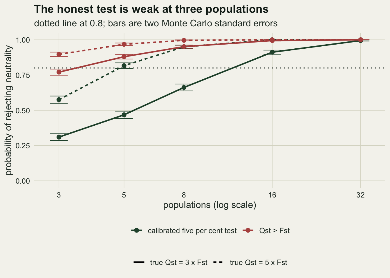
At 3 populations, a trait whose true Qst is three times Fst is detected by the calibrated test 31 per cent of the time, with a Monte Carlo standard error of 0.012. Push the divergence to five times Fst and the rate is 58 per cent. Going to 8 populations brings the threefold case to 66 per cent and 16 populations to 91 per cent. The point comparison looks much better on this figure, at 77 per cent at 3 populations, but its false-positive rate is 0.39 rather than 0.05, so the comparison is not a comparison of tests.
At 3 populations the study cannot support either conclusion. Use the point rule and a positive result carries a false-positive rate of 0.39; use the calibrated test instead and it misses 42 per cent of traits that really are five times more divergent than the markers. Comparisons resting on a handful of populations are common in this literature, as both Merila and Crnokrak’s compilation and the later review by Leinonen and colleagues record.
What to report
Report the number of populations first, and treat it as the sample size of the comparison. Individuals within populations buy precision on the within-population additive variance and on very little else; the among-population component has as many degrees of freedom as there are populations, minus one, whatever the total number of animals.
Report the breeding design and the variance components, not only the ratio. The nested mean squares and the components solved from them let a reader reconstruct Qst and check whether the among-population term was corrected for the sampling variance of the population means. A Qst quoted without the design behind it cannot be audited, and the bias measured above is large enough at small designs to change the conclusion by itself.
Give a critical value, not a comparison. Simulate the neutral distribution of Qst for the design and the estimated Fst in hand, quote its 95th percentile, and say whether the estimate exceeded it. If the estimate falls below that value, the honest statement is that neutrality is not rejected, which is different from a statement that the trait is neutral: the power figures above show how often a threefold divergence goes undetected. Say what Fst itself was estimated from, and treat it as a random quantity rather than a constant: the number of loci, the marker type and the estimator all move it, and a comparison that conditions on a point estimate of Fst, as this post does throughout, understates the total uncertainty.
Finally, report the negative results of the machinery. The fraction of replicates in which a variance component came out negative, or in which the ratio was truncated, is diagnostic. In the smallest design here, 8.5 per cent of neutral data sets returned a Qst of exactly one, which is what happens when the among-population component is positive and the estimated within-population additive variance comes out at or below zero, and 5.1 per cent returned exactly zero, which is what happens when the among-population component itself is non-positive. That case is tested first in qst_ratio, so a replicate with both components at or below zero is counted as a zero rather than as a one.
Honest limits
Fst is treated here as a known constant. It is not: it is estimated from a finite number of loci with its own sampling distribution, and the correct comparison is between two distributions rather than between an estimate and a point. Whitlock and Guillaume build that comparison properly. Carrying the marker-side uncertainty as well should widen the null, which would push the false-positive rates a study conditioning on a point estimate of Fst suffers above the ones reported here, but that is an argument and not a measurement: nothing in this post prices the marker side, so the size of the shift is unknown.
The demography is a star: populations that split simultaneously from one ancestor, drift independently at equal effective size, and exchange no migrants. Real populations are nested, unequal in size and connected, and correlated population means reduce the effective number of independent units below the count of sampling sites. The number of populations in the figures above should therefore be read as an upper bound on the information a real design of the same size carries.
The trait is purely additive with no dominance, no epistasis, no linkage and no genotype-by-environment interaction, and the common garden is assumed to have removed environmental divergence entirely. Dominance in particular pulls Qst below Fst under drift, which biases the comparison in the conservative direction for a test of divergent selection but in the anti-conservative direction for a test of stabilising selection. O’Hara and Merila work through the estimation problems that survive even under the additive model, and Leinonen and colleagues review the biological ones.
The alternative used for power is phenomenological. Scaling the population means to a target Qst reproduces the outcome of divergent selection without modelling the process, so the power figures apply to a trait that ended up that divergent, not to a specified strength of selection acting for a specified time. Power against a genuine selection model with the same mean divergence but different variance among populations would differ. The replicate counts behind all of this are 2500 for the null grid, 1500 for the design sweep and 1500 for the power runs, giving Monte Carlo standard errors of at most 0.010, 0.013 and 0.013 on any single rate. The critical multiples carry bootstrap standard errors reaching 0.33 at the smallest number of populations and the lowest Fst, which is where the null tail is longest and the 95th percentile is worst determined.
References
Lande R 1992 Evolution 46(2):381-389 (10.1111/j.1558-5646.1992.tb02046.x)
Spitze K 1993 Genetics 135(2):367-374 (10.1093/genetics/135.2.367)
Merila J, Crnokrak P 2001 Journal of Evolutionary Biology 14(6):892-903 (10.1046/j.1420-9101.2001.00348.x)
O’Hara RB, Merila J 2005 Genetics 171(3):1331-1339 (10.1534/genetics.105.044545)
Whitlock MC 2008 Molecular Ecology 17(8):1885-1896 (10.1111/j.1365-294X.2008.03712.x)
Whitlock MC, Guillaume F 2009 Genetics 183(3):1055-1063 (10.1534/genetics.108.099812)
Leinonen T, McCairns RJS, O’Hara RB, Merila J 2013 Nature Reviews Genetics 14(3):179-190 (10.1038/nrg3395)