library(ggplot2)

te_pal <- list(forest = "#275139", green = "#2f8f63", sage = "#93a87f",
               clay = "#b5534e", gold = "#cda23f", line = "#dad9ca",
               ink = "#16241d")

theme_te <- function() {
  theme_minimal(base_size = 12) +
    theme(panel.grid.minor = element_blank(),
          panel.grid.major = element_line(colour = "#e7e6dc"),
          plot.background = element_rect(fill = "#f5f4ee", colour = NA),
          panel.background = element_rect(fill = "#f5f4ee", colour = NA),
          plot.title = element_text(face = "bold", colour = te_pal$ink),
          axis.title = element_text(colour = "#2c3a31"))
}F-statistics and population structure
R
population genetics
ecology tutorial
ggplot2
Compute Fis, Fst and Fit in R from three heterozygosities, see why Gst is capped by diversity within populations, and estimate Fst without the sampling bias.
Corrected 14 October 2026: the introduction said the ceiling on Gst is why microsatellite and SNP studies of the same populations report values an order of magnitude apart, a factor the post’s own ceilings do not reach, and it now calls the ceiling a large part of the reason they can differ widely; and the descriptive ratio, called defensible whenever the populations are the whole question, is now called so only once enough individuals are sampled for its sampling bias to be small.
Corrected 30 September 2026: the post read a near-zero Fis at one locus as showing that each population mates at random; it now says the value is consistent with random mating, which is how the data were simulated.
The previous tutorial ended on an identity: pooling two subpopulations produced a heterozygote deficit exactly equal to twice the variance in allele frequency among them. Scale that variance by the largest it could be and you have Fst, the most used and most misread number in population genetics.
This tutorial does three things. It builds the hierarchy of Fis, Fst and Fit out of three heterozygosities. It then shows that Fst computed as a ratio of heterozygosities cannot exceed the homozygosity within populations, which is a large part of the reason microsatellite and SNP studies of the same populations can report very different values. Finally it swaps Nei’s descriptive ratio for the Weir and Cockerham estimator, and measures what that changes when samples are small.
Three heterozygosities, three F-statistics
Take five populations of one species along a gradient, 40 individuals genotyped in each at one biallelic locus, and allele frequencies that really do differ. Everything follows from three quantities: observed heterozygosity Ho, the mean expected heterozygosity within populations Hs, and the expected heterozygosity of the pooled gene pool Ht.
sim_pops <- function(p_vec, n_per, seed = NULL) {
  if (!is.null(seed)) set.seed(seed)
  t(sapply(p_vec, function(p)
    as.vector(rmultinom(1, n_per, c(p^2, 2 * p * (1 - p), (1 - p)^2)))))
}

f_stats <- function(geno) {
  n_i <- rowSums(geno)
  p_i <- (2 * geno[, 1] + geno[, 2]) / (2 * n_i)
  ho_i <- geno[, 2] / n_i
  hs <- mean(2 * p_i * (1 - p_i))
  p_bar <- mean(p_i)
  ht <- 2 * p_bar * (1 - p_bar)
  ho <- mean(ho_i)
  c(Ho = ho, Hs = hs, Ht = ht,
    Fis = 1 - ho / hs, Fst = 1 - hs / ht, Fit = 1 - ho / ht,
    var_p = mean((p_i - p_bar)^2), p_bar = p_bar)
}

geno <- sim_pops(c(0.15, 0.30, 0.45, 0.60, 0.80), 40, seed = 460)
dimnames(geno) <- list(paste0("pop", 1:5), c("AA", "AB", "BB"))
print(geno)
AA AB BB
pop1 1 9 30
pop2 2 19 19
pop3 10 16 14
pop4 16 16 8
pop5 17 21 2fs <- f_stats(geno)
print(round(fs, 4)) Ho Hs Ht Fis Fst Fit var_p p_bar
0.4050 0.4103 0.4909 0.0129 0.1641 0.1750 0.0403 0.4325 Fis is the shortfall of observed against within-population expectation, Fst the shortfall of within-population against total, and Fit the shortfall of observed against total. Each one is a deficit relative to a different reference, which is why they compose:
cat("(1 - Fit):", round(1 - fs[["Fit"]], 8),
    "  (1 - Fis)(1 - Fst):", round((1 - fs[["Fis"]]) * (1 - fs[["Fst"]]), 8), "\n")
(1 - Fit): 0.8250363 (1 - Fis)(1 - Fst): 0.8250363 print(all.equal(1 - fs[["Fit"]], (1 - fs[["Fis"]]) * (1 - fs[["Fst"]])))[1] TRUEcat("Fst as 1 - Hs/Ht:", round(fs[["Fst"]], 6),
" as var(p) / (pbar * qbar):",
round(fs[["var_p"]] / (fs[["p_bar"]] * (1 - fs[["p_bar"]])), 6), "\n")Fst as 1 - Hs/Ht: 0.164141 as var(p) / (pbar * qbar): 0.164141 In this sample Fis is 0.0129, Fst is 0.1641 and Fit is 0.1750, and the identity holds to machine precision. The second line is the connection to the previous tutorial: Fst computed from heterozygosities is numerically the same thing as the variance in allele frequency divided by its maximum, both 0.164141 here. One quantity, two readings: a deficit of heterozygotes, or a spread of allele frequencies.
Read Fis and Fst together. Here Fis is essentially zero, consistent with random mating within each population (which is how the genotypes were simulated); all the deficit relative to the total gene pool comes from the structure. Had these 200 individuals arrived as one unlabelled sample, the whole 0.175 would have been recorded as Fis and misread as inbreeding.
Gst cannot exceed the homozygosity within populations
The ratio 1 - Hs/Ht has an awkward property that gets it into trouble whenever marker types are compared. Consider the most extreme structure possible: five populations sharing no alleles at all, each with its own private set. Nothing could be more differentiated. Yet if each population is internally diverse, Hs is close to one, Ht cannot be much larger, and the ratio stays small.
ceiling_row <- function(k, d) {
  hs <- 1 - k * (1 / k)^2
  ht <- 1 - d * k * (1 / (k * d))^2
  gst <- (ht - hs) / ht
  gst_max <- (d - 1) * (1 - hs) / (d - 1 + hs)
  jost <- (ht - hs) / (1 - hs) * d / (d - 1)
  c(alleles_per_pop = k, Hs = hs, Ht = ht, Gst = gst,
    Gst_max = gst_max, Gprime_st = gst / gst_max, D = jost)
}

tab <- t(sapply(c(2, 5, 10, 20, 50), ceiling_row, d = 5))
print(round(tab, 4))
alleles_per_pop Hs Ht Gst Gst_max Gprime_st D
[1,] 2 0.50 0.900 0.4444 0.4444 1 1
[2,] 5 0.80 0.960 0.1667 0.1667 1 1
[3,] 10 0.90 0.980 0.0816 0.0816 1 1
[4,] 20 0.95 0.990 0.0404 0.0404 1 1
[5,] 50 0.98 0.996 0.0161 0.0161 1 1Five populations with no shared alleles and ten private alleles each give Gst = 0.0816. With 50 private alleles each it falls to 0.0161. The differentiation is total in every row; only the within-population diversity changes. Two rescalings fix the comparison: G'st divides by the maximum Gst attainable at that diversity, and Jost’s D measures the fraction of allelic diversity that is not shared. Both return exactly 1 in every row, which is the right answer for populations with no alleles in common.
sweep_k <- t(sapply(2:100, ceiling_row, d = 5))
plot_df <- data.frame(
  Hs = rep(sweep_k[, "Hs"], 3),
  value = c(sweep_k[, "Gst"], sweep_k[, "Gprime_st"], sweep_k[, "D"]),
  measure = rep(c("Gst", "G'st", "Jost D"), each = nrow(sweep_k)))

ggplot(plot_df, aes(Hs, value, colour = measure, linetype = measure)) +
  geom_line(linewidth = 0.9) +
  scale_colour_manual(values = c(Gst = te_pal$clay, `G'st` = te_pal$gold,
                                 `Jost D` = te_pal$forest), name = NULL) +
  scale_linetype_manual(values = c(Gst = "solid", `G'st` = "solid",
                                   `Jost D` = "dashed"), name = NULL) +
  labs(title = "Complete differentiation, three different answers",
       subtitle = "five populations, no shared alleles, only within-population diversity varies",
       x = "within-population expected heterozygosity Hs",
       y = "differentiation measure") +
  theme_te()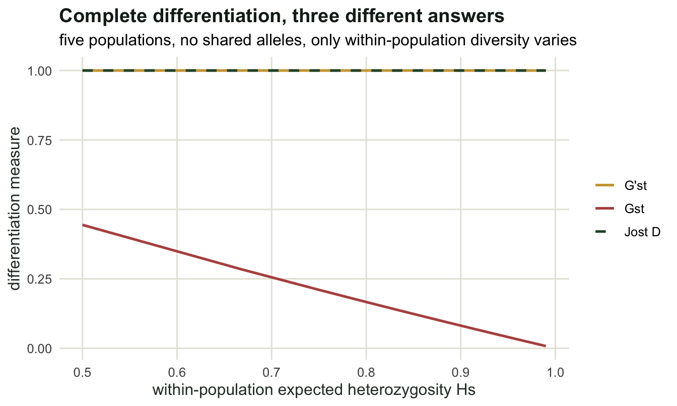
This is a large part of the reason a microsatellite study and a SNP study of the same populations disagree. Microsatellites carry Hs near 0.8, so their Gst is confined below about 0.17; SNPs carry Hs near 0.3, leaving room for much larger values. Neither marker is right. The number being reported is a ratio whose ceiling moved.
The practical rule is unglamorous: Fst and Gst answer “how much of the variance sits among populations”, which is the correct question for drift and migration, and they are the right statistics when the reference is a model. D answers “how different are the allele pools”, which is the correct question for comparing differentiation across marker types or across studies. Report the one that matches the question, and never compare Gst across marker sets without rescaling.
An estimator, not a description
Nei’s Gst is a description of the sample. With small samples that is a problem, because two populations drawn from an identical gene pool will differ by luck, and the ratio counts that luck as structure. Weir and Cockerham’s theta estimates the parameter instead: it partitions the variance into among-population, among-individual and within-individual components (their a, b and c) and corrects for sample size.
wc_theta <- function(geno) {
  n_i <- rowSums(geno)
  r <- nrow(geno)
  p_i <- (2 * geno[, 1] + geno[, 2]) / (2 * n_i)
  h_i <- geno[, 2] / n_i
  n_bar <- mean(n_i)
  n_c <- (r * n_bar - sum(n_i^2) / (r * n_bar)) / (r - 1)
  p_w <- sum(n_i * p_i) / (r * n_bar)
  s2 <- sum(n_i * (p_i - p_w)^2) / ((r - 1) * n_bar)
  h_w <- sum(n_i * h_i) / (r * n_bar)
  a <- n_bar / n_c * (s2 - (p_w * (1 - p_w) - (r - 1) / r * s2 - h_w / 4) /
                        (n_bar - 1))
  b <- n_bar / (n_bar - 1) * (p_w * (1 - p_w) - (r - 1) / r * s2 -
                                (2 * n_bar - 1) / (4 * n_bar) * h_w)
  cw <- h_w / 2
  c(a = a, b = b, c = cw, theta = a / (a + b + cw))
}

print(round(wc_theta(geno), 4))
a b c theta
0.0477 0.0053 0.2025 0.1867 cat("Nei Gst:", round(fs[["Fst"]], 4),
" rescaled by r/(r - 1):", round(fs[["Fst"]] * 5 / 4, 4), "\n")Nei Gst: 0.1641 rescaled by r/(r - 1): 0.2052 On the five-population sample theta is 0.1867 while Nei’s Gst is 0.1641, and the gap is not sampling error: 40 individuals per population is plenty. Two differences are at work. The estimator divides the among-population sum of squares by one less than the number of populations, treating these five populations as a sample from a wider set rather than as the entire world, which alone rescales 0.1641 to 0.2052. It then subtracts the variance expected from sampling 40 individuals from the among-population component and, in the denominator, replaces the sample’s own total variance with a slightly larger estimate for the wider set of populations; together those pull the value back down to 0.1867. Nei’s ratio describes these five populations; theta estimates the parameter of the process that produced them. When the populations are the whole question (five islands, and there are five islands), the descriptive ratio is a defensible choice once enough individuals are sampled for its sampling bias, measured below, to be small; when they are a sample from a species range, it is not.
The correction matters most when samples are small. Draw every population from the same allele frequency, so the true Fst is zero by construction, and see what each measure reports.
sim_flat <- function(n_per, r = 5, p = 0.4) {
  t(sapply(seq_len(r), function(i)
    as.vector(rmultinom(1, n_per, c(p^2, 2 * p * (1 - p), (1 - p)^2)))))
}

set.seed(464)
n_loci <- 3000

sweep_n <- function(n) {
  out <- t(sapply(seq_len(n_loci), function(i) {
    g <- sim_flat(n)
    wc <- wc_theta(g)
    c(f_stats(g)[["Fst"]], wc[["a"]], sum(wc[c("a", "b", "c")]))
  }))
  c(n_per_pop = n, mean_Gst = mean(out[, 1]),
    theta = sum(out[, 2]) / sum(out[, 3]))
}

bias <- t(sapply(c(5, 10, 25, 50, 100), sweep_n))
print(round(bias, 4))
n_per_pop mean_Gst theta
[1,] 5 0.0814 -7e-04
[2,] 10 0.0399 -4e-04
[3,] 25 0.0162 2e-04
[4,] 50 0.0079 -1e-04
[5,] 100 0.0040 0e+00With five individuals per population and no structure whatsoever, Nei’s Gst reports 0.0814. At ten individuals it is 0.0399, at 25 it is 0.0162, at 50 it is 0.0079 and at 100 it is 0.0040: the bias halves as the sample size doubles, tracking (r - 1)/(2nr), which with five populations is 0.4/n. The Weir and Cockerham estimator stays between -0.0007 and 0.0002 across the same range. Ten individuals per population is a very ordinary design, and it manufactures an Fst of 0.04 out of nothing.
bias_df <- data.frame(
  n = rep(bias[, "n_per_pop"], 2),
  value = c(bias[, "mean_Gst"], bias[, "theta"]),
  measure = rep(c("Nei Gst", "Weir and Cockerham theta"), each = nrow(bias)))

ggplot(bias_df, aes(n, value, colour = measure)) +
  geom_hline(yintercept = 0, colour = te_pal$line) +
  geom_line(data = data.frame(n = 5:100, value = (5 - 1) / (2 * (5:100) * 5),
                              measure = "(r-1)/(2nr)"),
            linetype = "dashed", colour = "grey55", linewidth = 0.7) +
  geom_line(linewidth = 0.9) +
  geom_point(size = 2.2) +
  scale_x_log10(breaks = c(5, 10, 25, 50, 100)) +
  scale_colour_manual(values = c(`Nei Gst` = te_pal$clay,
                                 `Weir and Cockerham theta` = te_pal$forest,
                                 `(r-1)/(2nr)` = "grey55"), name = NULL) +
  labs(title = "True Fst is zero in every one of these simulations",
       subtitle = "5 populations, 3000 biallelic loci per point",
       x = "individuals per population (log scale)",
       y = "measured differentiation") +
  theme_te()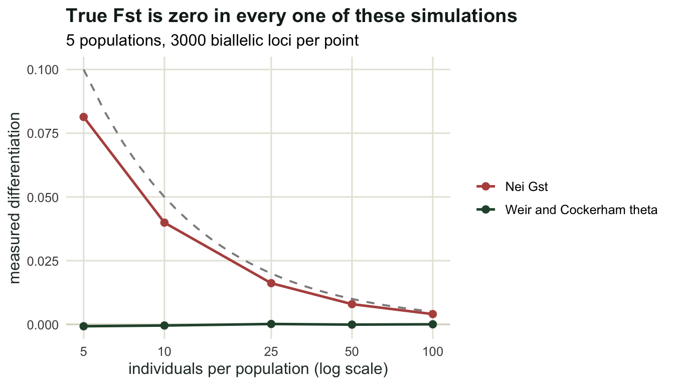
One locus tells you almost nothing
Now give the simulation a real parameter. Balding and Nichols’ beta model draws each population’s allele frequency around an ancestral value with a spread set by Fst, which is the standard way to generate data with a known answer.
bn_draw <- function(p, fst) {
  rbeta(1, p * (1 - fst) / fst, (1 - p) * (1 - fst) / fst)
}

sim_struct <- function(n_per, r, p, fst) {
  ps <- replicate(r, bn_draw(p, fst))
  t(sapply(ps, function(pp)
    as.vector(rmultinom(1, n_per, c(pp^2, 2 * pp * (1 - pp), (1 - pp)^2)))))
}

set.seed(463)
n_loci <- 2000
per_locus <- t(sapply(seq_len(n_loci), function(i) {
  g <- sim_struct(50, 10, 0.3, 0.05)
  wc <- wc_theta(g)
  c(gst = f_stats(g)[["Fst"]], theta = wc[["theta"]], a = wc[["a"]],
    abc = sum(wc[c("a", "b", "c")]))
}))

cat("true Fst 0.05, 10 populations, 50 individuals each\n")
true Fst 0.05, 10 populations, 50 individuals eachcat("theta as ratio of averages:",
round(sum(per_locus[, "a"]) / sum(per_locus[, "abc"]), 4),
" mean per-locus theta:", round(mean(per_locus[, "theta"]), 4),
" mean Gst:", round(mean(per_locus[, "gst"]), 4), "\n")theta as ratio of averages: 0.0505 mean per-locus theta: 0.0502 mean Gst: 0.0541 cat("per-locus theta: sd", round(sd(per_locus[, "theta"]), 4),
" fraction negative", round(mean(per_locus[, "theta"] < 0), 4), "\n")per-locus theta: sd 0.0263 fraction negative 0.0015 print(round(quantile(per_locus[, "theta"], c(0.05, 0.5, 0.95)), 4)) 5% 50% 95%
0.0132 0.0468 0.1003 The multilocus estimate is 0.0505 against a true 0.05. Single loci are another matter: the standard deviation across loci is 0.0263, the central 90 per cent of loci fall between 0.0132 and 0.1003, and 0.15 per cent of them come out negative. A negative Fst is not an error to be truncated at zero; it is the estimator telling you that this locus has less among-population variance than the sampling noise, which is rare at this true value and these sample sizes but common when the true value is close to zero.
ggplot(data.frame(theta = per_locus[, "theta"]), aes(theta)) +
  geom_histogram(bins = 60, fill = te_pal$sage, colour = "white") +
  geom_vline(xintercept = 0.05, colour = te_pal$clay, linewidth = 0.9) +
  labs(title = "One locus is a very noisy estimate of Fst",
       subtitle = "true Fst 0.05, red line at the truth",
       x = "per-locus Weir and Cockerham estimate", y = "loci") +
  theme_te()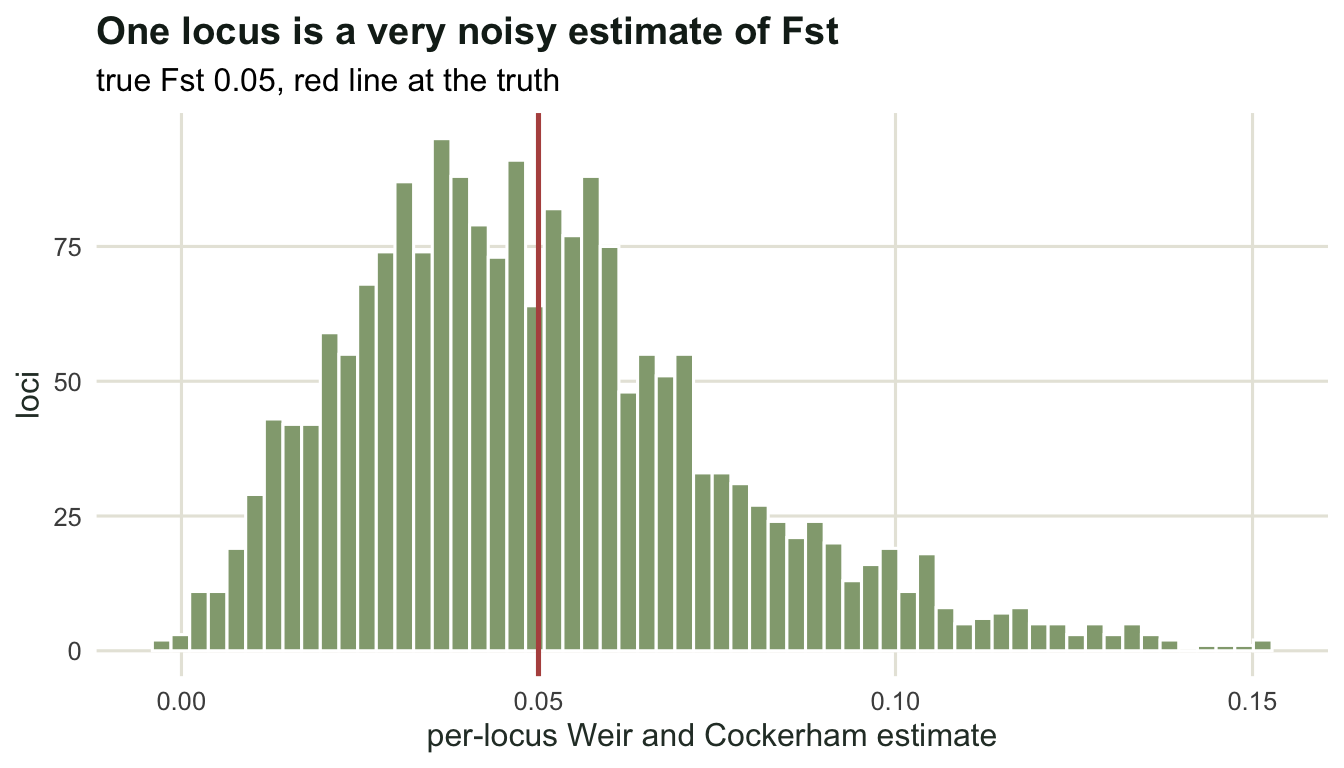
That noise also settles how loci should be combined. The estimator is a ratio, and ratios do not average: sum the numerators and the denominators over loci, then divide once. Averaging per-locus ratios is a different quantity, and with rare alleles it misbehaves badly.
set.seed(465)
n_loci <- 3000
mixed <- t(sapply(seq_len(n_loci), function(i) {
  p0 <- runif(1, 0.02, 0.5)
  g <- sim_struct(20, 5, p0, 0.05)
  wc <- wc_theta(g)
  c(theta = wc[["theta"]], a = wc[["a"]], abc = sum(wc[c("a", "b", "c")]),
    p = p0)
}))

undef <- !is.finite(mixed[, "theta"])
cat("loci with an undefined per-locus ratio:", sum(undef), "of", n_loci,
    " mean allele frequency of those loci:",
    round(mean(mixed[undef, "p"]), 4), "\n")
loci with an undefined per-locus ratio: 8 of 3000 mean allele frequency of those loci: 0.0294 cat("ratio of averages:",
round(sum(mixed[, "a"]) / sum(mixed[, "abc"]), 4),
" average of per-locus ratios (undefined dropped):",
round(mean(mixed[!undef, "theta"]), 4),
" median per-locus ratio:", round(median(mixed[!undef, "theta"]), 4), "\n")ratio of averages: 0.0494 average of per-locus ratios (undefined dropped): 0.0463 median per-locus ratio: 0.0351 Eight of 3000 loci have no ratio at all, because a locus that came out monomorphic in the sample has zero in every variance component and 0/0 is undefined. Their mean allele frequency was 0.0294, so they are exactly the rare variants a real data set contains in quantity. The ratio of averages ignores the problem and returns 0.0494 against a truth of 0.05. Averaging the defined ratios gives 0.0463, and the median per-locus value is 0.0351, which is 30 per cent low. The rule is one line of arithmetic and it is not optional.
Where to go next
Fst has been treated as a description so far: this much of the variance sits among populations. It is more useful than that, because population genetic theory predicts the value from drift and gene flow, which turns a measured Fst into a statement about how connected the populations are. The next tutorial simulates that machinery, checks the classic 1/(1 + 4Nm) result against a simulation, and then looks hard at how much a measured Fst really licenses you to say about migration.
References
Wright S 1951 Annals of Eugenics 15(4):323-354 (10.1111/j.1469-1809.1949.tb02451.x)
Nei M 1973 Proceedings of the National Academy of Sciences 70(12):3321-3323 (10.1073/pnas.70.12.3321)
Weir BS, Cockerham CC 1984 Evolution 38(6):1358-1370 (10.1111/j.1558-5646.1984.tb05657.x)
Hedrick PW 2005 Evolution 59(8):1633-1638 (10.1111/j.0014-3820.2005.tb01814.x)
Jost L 2008 Molecular Ecology 17(18):4015-4026 (10.1111/j.1365-294X.2008.03887.x)
Meirmans PG, Hedrick PW 2011 Molecular Ecology Resources 11(1):5-18 (10.1111/j.1755-0998.2010.02927.x)
Bhatia G, Patterson N, Sankararaman S, Price AL 2013 Genome Research 23(9):1514-1521 (10.1101/gr.154831.113)
Balding DJ, Nichols RA 1995 Genetica 96(1-2):3-12 (10.1007/BF01441146)