library(ggplot2)

te_pal <- list(forest = "#275139", green = "#2f8f63", sage = "#93a87f",
               clay = "#b5534e", gold = "#cda23f", line = "#dad9ca",
               ink = "#16241d")

theme_te <- function() {
  theme_minimal(base_size = 12) +
    theme(panel.grid.minor = element_blank(),
          panel.grid.major = element_line(colour = "#e7e6dc"),
          plot.background = element_rect(fill = "#f5f4ee", colour = NA),
          panel.background = element_rect(fill = "#f5f4ee", colour = NA),
          plot.title = element_text(face = "bold", colour = te_pal$ink),
          axis.title = element_text(colour = "#2c3a31"))
}Checking a population genetics analysis
R
population genetics
model diagnostics
ecology tutorial
ggplot2
Four checks for an Fst analysis in R: loci against individuals, separating substructure from marker error, filtering rare variants, and outlier tests.
Corrected 1 October 2026: Check two said its two scenarios were built to give almost the same mean Fis and that every other summary tells them apart; they only happen to match in this draw, and the post now says the extreme loci are the dependable footprint, since the shift under substructure is small against the scatter of a single locus. Check three put the filtering effect down to rare loci having little variance to divide up; it now says the filter selects on the same frequencies the estimate is built from, keeping rare variants that drifted up and discarding those that drifted least.
Corrected 30 September 2026: Check 1 said that above a small floor it makes no difference whether genotypes come from many individuals or many loci; with a fixed number of loci the among-locus variation in drift limits what extra individuals can buy, and the post now says the product rule holds only for modest sample sizes.
The three tutorials before this one worked with data whose answer was known. That is the only way to learn what an estimator does, and it is also why the numbers came out reassuring. This one is about the checks that stay useful when the answer is not known, which is every real project.
Four checks, in the order they usually matter: whether the design has enough information, whether a positive Fis is biology or a marker problem, what a routine filtering step does to the estimate, and whether an outlier locus means selection. Each one is a simulation with a known truth, run so that the diagnostic can be calibrated before it is trusted.
Two helpers carry the whole post. The first simulates many biallelic loci in several populations with a known Fst, using the beta model from the second tutorial and drawing genotype counts directly. The second is the Weir and Cockerham estimator, vectorised across loci, combining them as a ratio of averages.
sim_loci <- function(n_loci, r, n_ind, fst, p_anc) {
  if (length(p_anc) == 1) p_anc <- rep(p_anc, n_loci)
  aa <- ab <- bb <- matrix(0L, n_loci, r)
  shape1 <- p_anc * (1 - fst) / fst
  shape2 <- (1 - p_anc) * (1 - fst) / fst
  for (j in seq_len(r)) {
    p_j <- rbeta(n_loci, shape1, shape2)
    het <- rbinom(n_loci, n_ind, 2 * p_j * (1 - p_j))
    rest <- n_ind - het
    hom_a <- rbinom(n_loci, rest, p_j^2 / (p_j^2 + (1 - p_j)^2))
    aa[, j] <- hom_a
    ab[, j] <- het
    bb[, j] <- rest - hom_a
  }
  list(aa = aa, ab = ab, bb = bb, n = n_ind, r = r)
}

wc_multi <- function(g) {
  n <- g$n
  r <- g$r
  p <- (2 * g$aa + g$ab) / (2 * n)
  h <- g$ab / n
  p_w <- rowMeans(p)
  s2 <- rowSums((p - p_w)^2) / (r - 1)
  h_w <- rowMeans(h)
  a <- s2 - (p_w * (1 - p_w) - (r - 1) / r * s2 - h_w / 4) / (n - 1)
  b <- n / (n - 1) * (p_w * (1 - p_w) - (r - 1) / r * s2 -
                        (2 * n - 1) / (4 * n) * h_w)
  cw <- h_w / 2
  list(theta = sum(a) / sum(a + b + cw), per_locus = a / (a + b + cw))
}
Check 1: loci or individuals?
Field time buys individuals and laboratory budget buys loci, and the two are not interchangeable. Fix the truth at Fst = 0.05 in five populations and measure the precision of the multilocus estimate across a grid.
set.seed(471)

n_rep <- 200
design <- expand.grid(n_ind = c(2, 4, 8, 16, 32), n_loci = c(10, 100, 1000))
design$mean_theta <- NA_real_
design$sd_theta <- NA_real_
for (k in seq_len(nrow(design))) {
  est <- replicate(n_rep, wc_multi(sim_loci(design$n_loci[k], 5,
                                            design$n_ind[k], 0.05, 0.3))$theta)
  design$mean_theta[k] <- mean(est)
  design$sd_theta[k] <- sd(est)
}
design$sd_times_root_nL <- design$sd_theta * sqrt(design$n_ind * design$n_loci)
print(round(design, 4))
n_ind n_loci mean_theta sd_theta sd_times_root_nL
1 2 10 0.0547 0.0763 0.3413
2 4 10 0.0464 0.0396 0.2505
3 8 10 0.0499 0.0242 0.2162
4 16 10 0.0493 0.0170 0.2156
5 32 10 0.0502 0.0130 0.2333
6 2 100 0.0509 0.0257 0.3634
7 4 100 0.0517 0.0133 0.2657
8 8 100 0.0504 0.0078 0.2212
9 16 100 0.0501 0.0053 0.2133
10 32 100 0.0499 0.0043 0.2405
11 2 1000 0.0489 0.0071 0.3164
12 4 1000 0.0497 0.0035 0.2245
13 8 1000 0.0498 0.0024 0.2185
14 16 1000 0.0500 0.0016 0.2011
15 32 1000 0.0501 0.0013 0.2395Two things to read off. First, the mean estimate is centred on the truth in every cell, from 0.0464 to 0.0547 across the whole grid and from 0.0489 to 0.0517 once there are 100 loci, including the cells with two individuals per population: the estimator is unbiased regardless of sample size, which is the property Nei’s ratio lacked. Only the scatter changes.
Second, the scatter is governed by the product. The last column is the standard deviation multiplied by the square root of the number of genotypes, and from four individuals upward it sits between 0.2011 and 0.2657 everywhere in the grid, across designs whose smallest and largest differ by nearly three orders of magnitude in size. Precision therefore comes from n * L, and the design question becomes which factor is cheaper to raise. Two individuals do pay a penalty (0.3164 to 0.3634), so a floor of about four individuals per population is worth respecting. Above that floor the product rule holds only while the number of individuals stays modest: at every number of loci the product already rises between 16 and 32 individuals, because with a fixed number of loci the variation in drift among loci sets a floor that more individuals cannot remove. Beyond a few tens of individuals per population, extra loci buy far more precision than extra individuals.
ggplot(design, aes(n_loci, sd_theta, colour = factor(n_ind))) +
  geom_line(linewidth = 0.9) +
  geom_point(size = 2) +
  scale_x_log10(breaks = c(10, 100, 1000)) +
  scale_y_log10() +
  scale_colour_manual(values = c(`2` = te_pal$clay, `4` = te_pal$gold,
                                 `8` = te_pal$sage, `16` = te_pal$green,
                                 `32` = te_pal$forest),
                      name = "individuals\nper population") +
  labs(title = "Precision follows the number of genotypes",
       subtitle = "true Fst 0.05, five populations, 200 replicates per point",
       x = "loci (log scale)", y = "SD of the estimate (log scale)") +
  theme_te()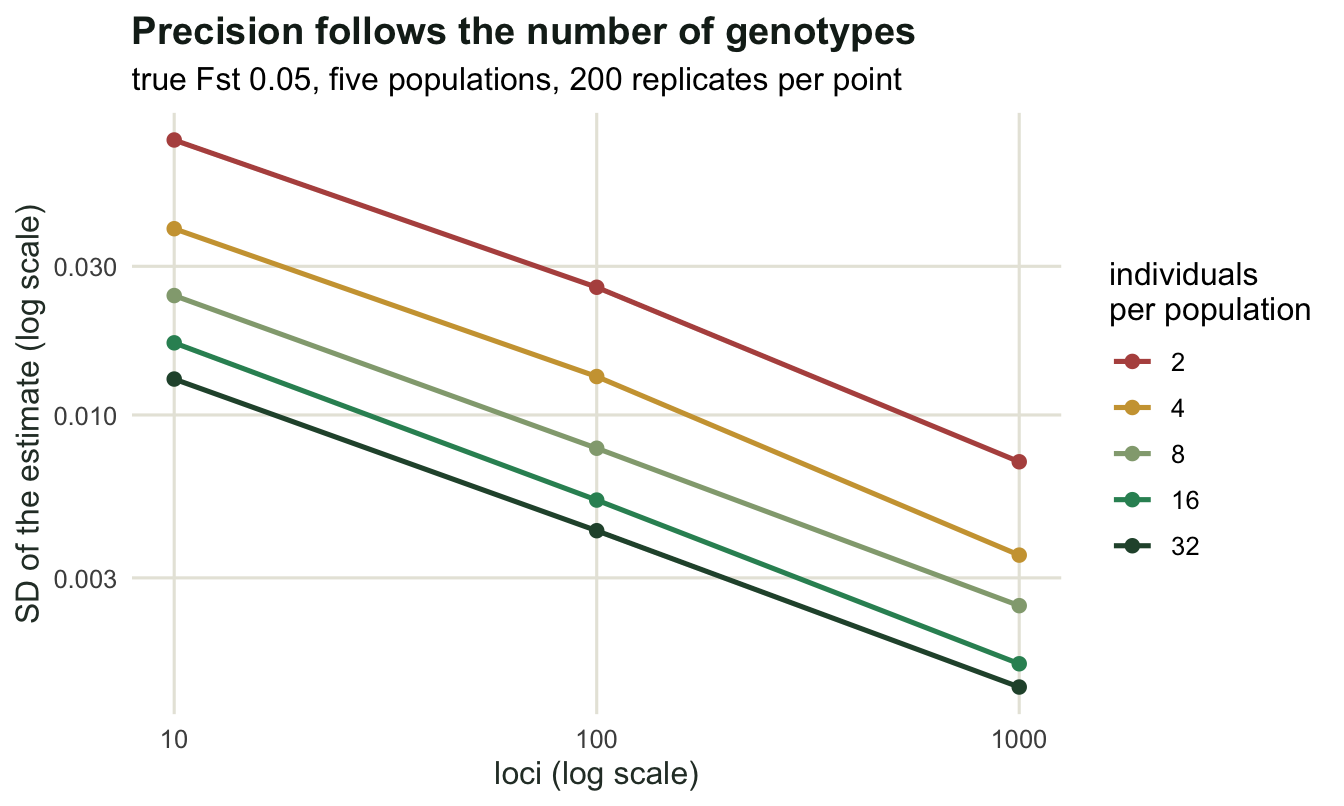
The caveat is the part the simulation cannot show. Here every locus receives its own independent draw of population history, so adding loci keeps shrinking the error without limit. Real loci share one history and are linked into blocks, so beyond a few thousand markers the error stops falling: what remains is the uncertainty of the single realised history, and no amount of sequencing removes it. Treat the grid as an upper bound on what loci buy.
Check 2: is that Fis biology or a pipette?
A positive Fis was ambiguous in the first tutorial: population structure and allelic dropout produce the same heterozygote deficit. With more than one locus the ambiguity is resolvable, because the two mechanisms leave different footprints across loci. Structure shifts every locus a little; a marker artefact wrecks a few loci badly.
Both scenarios below happen to give almost the same mean Fis in this draw, which is what makes the point.
fis_per_locus <- function(aa, ab, bb) {
  n <- aa + ab + bb
  p <- (2 * aa + ab) / (2 * n)
  1 - (ab / n) / (2 * p * (1 - p))
}

set.seed(472)
n_loci <- 100
n_ind <- 400

## scenario A: one sample that is really two subpopulations, Fst 0.015
fst_sub <- 0.015
p_anc <- runif(n_loci, 0.15, 0.5)
sh1 <- p_anc * (1 - fst_sub) / fst_sub
sh2 <- (1 - p_anc) * (1 - fst_sub) / fst_sub
p1 <- rbeta(n_loci, sh1, sh2)
p2 <- rbeta(n_loci, sh1, sh2)

mix_geno <- function(p_a, p_b, n_half) {
  het <- rbinom(length(p_a), n_half, 2 * p_a * (1 - p_a)) +
    rbinom(length(p_b), n_half, 2 * p_b * (1 - p_b))
  hom_a <- rbinom(length(p_a), n_half, p_a^2) +
    rbinom(length(p_b), n_half, p_b^2)
  cbind(aa = hom_a, ab = het, bb = 2 * n_half - hom_a - het)
}

sub_dat <- mix_geno(p1, p2, n_ind / 2)
fis_sub <- fis_per_locus(sub_dat[, "aa"], sub_dat[, "ab"], sub_dat[, "bb"])

## scenario B: random mating, but five loci lose 30 per cent of heterozygotes
het <- rbinom(n_loci, n_ind, 2 * p_anc * (1 - p_anc))
hom_a <- rbinom(n_loci, n_ind - het, p_anc^2 / (p_anc^2 + (1 - p_anc)^2))
hom_b <- n_ind - het - hom_a
bad <- 1:5
lost <- rbinom(length(bad), het[bad], 0.3)
lost_a <- rbinom(length(bad), lost, 0.5)
het[bad] <- het[bad] - lost
hom_a[bad] <- hom_a[bad] + lost_a
hom_b[bad] <- hom_b[bad] + lost - lost_a
fis_art <- fis_per_locus(hom_a, het, hom_b)

report <- function(x, label) {
  cat(label, " mean", round(mean(x), 4), " median", round(median(x), 4),
      " sd", round(sd(x), 4), " max", round(max(x), 4),
      " loci above 0.15:", sum(x > 0.15),
      " loci above zero:", sum(x > 0), "\n")
}
report(fis_sub, "hidden substructure:")
hidden substructure: mean 0.0107 median 0.0156 sd 0.0515 max 0.1146 loci above 0.15: 0 loci above zero: 59 report(fis_art, "dropout at 5 loci: ")dropout at 5 loci: mean 0.0123 median -0.005 sd 0.0881 max 0.3824 loci above 0.15: 5 loci above zero: 48 cat("the five damaged loci:", round(fis_art[bad], 3), "\n")the five damaged loci: 0.364 0.295 0.382 0.211 0.332 cat("the other 95 loci: mean", round(mean(fis_art[-bad]), 4),
" median", round(median(fis_art[-bad]), 4), "\n")the other 95 loci: mean -0.0037 median -0.0089 Mean Fis is 0.0107 under hidden substructure and 0.0123 under dropout, so a report that quotes only the mean cannot distinguish them. The per-locus values can. Under substructure the median is 0.0156, positive like the mean, 59 of 100 loci are above zero, and the largest single value is 0.1146. Under dropout the median is -0.005, the undamaged 95 loci average -0.0037, and the five broken loci come in at 0.211 to 0.382. The dependable difference is the five extreme loci: the upward shift under substructure is small against the scatter of a single locus, and this draw shows it more clearly than most draws of the same design would.
fis_df <- data.frame(
  locus = rep(1:n_loci, 2),
  fis = c(fis_sub, fis_art),
  scenario = rep(c("hidden substructure", "dropout at 5 loci"),
                 each = n_loci))
fis_df$scenario <- factor(fis_df$scenario,
                          levels = c("hidden substructure",
                                     "dropout at 5 loci"))

ggplot(fis_df, aes(locus, fis)) +
  geom_hline(yintercept = 0, colour = te_pal$line) +
  geom_point(aes(colour = scenario), size = 1.7, show.legend = FALSE) +
  facet_wrap(~scenario) +
  scale_colour_manual(values = c(`hidden substructure` = te_pal$forest,
                                 `dropout at 5 loci` = te_pal$clay)) +
  labs(title = "Same mean Fis, different footprint across loci",
       subtitle = "100 loci, 400 individuals",
       x = "locus", y = "per-locus Fis") +
  theme_te()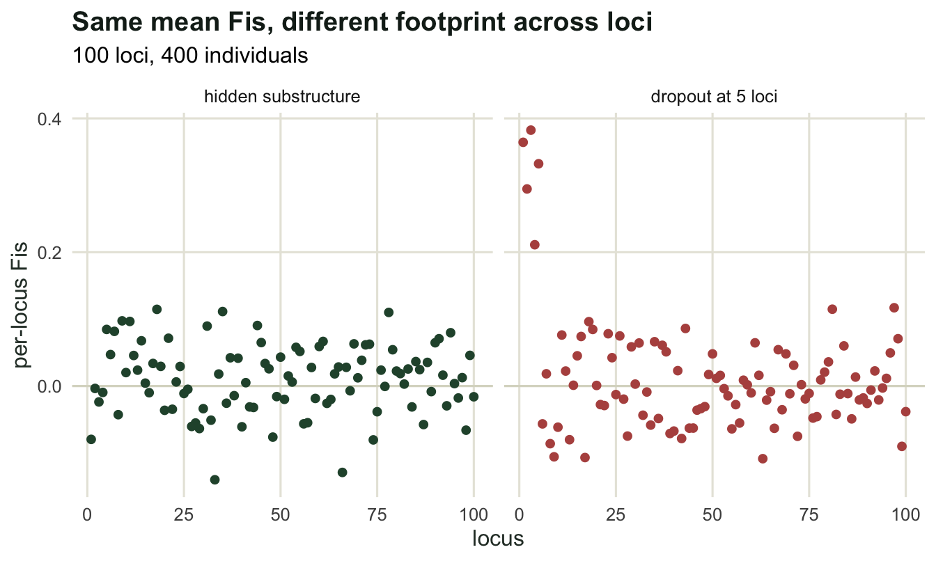
The check is therefore to plot Fis per locus and never to average first. A shifted cloud says the sample is not one randomly mating population, and the remedy is to look for the grouping. A flat cloud with a few extreme loci says those loci are broken, and the remedy is to drop them. A biologically inbred population gives the shifted cloud too, so this check narrows the possibilities to two rather than one; separating true inbreeding from unrecognised structure needs the sampling design, not the genotypes.
Check 3: what filtering rare variants does
Almost every pipeline discards markers below a minor allele frequency threshold. That step is not neutral for Fst, because the filter reads the same allele frequencies that Fst is computed from. Simulate a realistic frequency spectrum with many rare variants, then estimate Fst on the whole set and on the filtered set.
set.seed(473)

p_spec <- 1 / seq(2, 40)                 # 0.5 down to 0.025, no fixed sites
p_spec <- sample(p_spec, 4000, replace = TRUE)
g_all <- sim_loci(4000, 5, 25, 0.05, p_spec)

p_pooled <- rowMeans((2 * g_all$aa + g_all$ab) / (2 * g_all$n))
maf <- pmin(p_pooled, 1 - p_pooled)
keep <- maf >= 0.05

subset_g <- function(g, idx) {
  list(aa = g$aa[idx, ], ab = g$ab[idx, ], bb = g$bb[idx, ], n = g$n, r = g$r)
}

cat("all loci:", nrow(g_all$aa),
    " theta:", round(wc_multi(g_all)$theta, 4), "\n")
all loci: 4000 theta: 0.0481 cat("loci kept at MAF 0.05:", sum(keep),
" theta:", round(wc_multi(subset_g(g_all, keep))$theta, 4), "\n")loci kept at MAF 0.05: 2053 theta: 0.0518 cat("loci discarded:", sum(!keep),
" theta:", round(wc_multi(subset_g(g_all, !keep))$theta, 4), "\n")loci discarded: 1947 theta: 0.0312 The truth is 0.05 and the full set returns 0.0481. Filtering at a minor allele frequency of 0.05 throws away 1947 of 4000 loci and returns 0.0518, eight per cent above the unfiltered estimate, while the discarded loci on their own give 0.0312. The cause is not rarity as such: in this simulation every locus has the same true Fst, whatever its ancestral frequency. It is that the filter reads the same pooled frequencies the estimate is built from. A variant that is rare in the ancestral pool clears the threshold mainly when drift or sampling has carried it up in one or more populations, which is when it looks most differentiated, while the rare variants left below the threshold are mostly those that drifted least. Filtering keeps the first kind and discards the second, so the kept set reads high and the discarded set reads low.
The consequence is a comparability rule. An Fst from a filtered SNP set is not on the same scale as an Fst from an unfiltered one, and a threshold applied to the pooled sample is not the same as a threshold applied per population. When two studies of the same species disagree about Fst, the filtering step is one of the first places to look, alongside the marker type argument from the second tutorial.
Check 4: an outlier is only an outlier under a model
Fst outlier scans look for loci more differentiated than a neutral null and call them candidates for selection. The scan is only as good as the null, and the usual null is an island model in which every population is equally related to every other. Real sampling rarely looks like that: populations fall into regions, catchments, or lineages.
Simulate two groups of three demes, with real structure among the groups and very little within them, and no selection anywhere. Then run the standard scan with an island-model null calibrated to the same overall Fst.
set.seed(474)

hier <- function(n_loci, n_ind, fst_among, fst_within, p_anc) {
  sh1 <- p_anc * (1 - fst_among) / fst_among
  sh2 <- (1 - p_anc) * (1 - fst_among) / fst_among
  out_aa <- out_ab <- out_bb <- matrix(0L, n_loci, 6)
  for (grp in 1:2) {
    p_grp <- rbeta(n_loci, sh1, sh2)
    s1 <- p_grp * (1 - fst_within) / fst_within
    s2 <- (1 - p_grp) * (1 - fst_within) / fst_within
    for (d in 1:3) {
      col <- (grp - 1) * 3 + d
      p_d <- rbeta(n_loci, s1, s2)
      het <- rbinom(n_loci, n_ind, 2 * p_d * (1 - p_d))
      rest <- n_ind - het
      hom_a <- rbinom(n_loci, rest, p_d^2 / (p_d^2 + (1 - p_d)^2))
      out_aa[, col] <- hom_a
      out_ab[, col] <- het
      out_bb[, col] <- rest - hom_a
    }
  }
  list(aa = out_aa, ab = out_ab, bb = out_bb, n = n_ind, r = 6)
}

p_base <- runif(2000, 0.1, 0.5)
obs <- hier(2000, 30, 0.08, 0.01, p_base)
obs_fit <- wc_multi(obs)
cat("hierarchical data, multilocus theta:", round(obs_fit$theta, 4), "\n")
hierarchical data, multilocus theta: 0.0592 null_g <- sim_loci(20000, 6, 30, obs_fit$theta, sample(p_base, 20000, TRUE))
null_per <- wc_multi(null_g)$per_locus
thr <- quantile(null_per, 0.99, na.rm = TRUE)
cat("island-model null, 99th percentile of per-locus theta:",
round(thr, 4), "\n")island-model null, 99th percentile of per-locus theta: 0.1949 cat("hierarchical loci above that threshold:",
round(mean(obs_fit$per_locus > thr), 4),
" nominal rate: 0.01\n")hierarchical loci above that threshold: 0.048 nominal rate: 0.01cat("null spread: sd", round(sd(null_per), 4),
" hierarchical spread: sd", round(sd(obs_fit$per_locus), 4), "\n")null spread: sd 0.0445 hierarchical spread: sd 0.067 Not one locus in this simulation is under selection. The scan flags 4.8 per cent of them, nearly five times the nominal one per cent, because the hierarchical arrangement widens the distribution of per-locus Fst beyond what the island model expects (standard deviation 0.067 against 0.0445). Every flagged locus would be reported as a candidate, and a gene ontology analysis of the list would find something to say about it.
dens_df <- data.frame(
  theta = c(null_per, obs_fit$per_locus),
  model = rep(c("island-model null", "hierarchical truth"),
              c(length(null_per), length(obs_fit$per_locus))))

ggplot(dens_df, aes(theta, colour = model)) +
  geom_density(linewidth = 0.9) +
  geom_vline(xintercept = thr, linetype = "dashed", colour = "grey40") +
  coord_cartesian(xlim = c(-0.05, 0.45)) +
  scale_colour_manual(values = c(`island-model null` = te_pal$sage,
                                 `hierarchical truth` = te_pal$clay),
                      name = NULL) +
  labs(title = "The same overall Fst, a heavier tail",
       subtitle = "dashed line: 99th percentile of the island-model null",
       x = "per-locus Weir and Cockerham estimate", y = "density") +
  theme_te()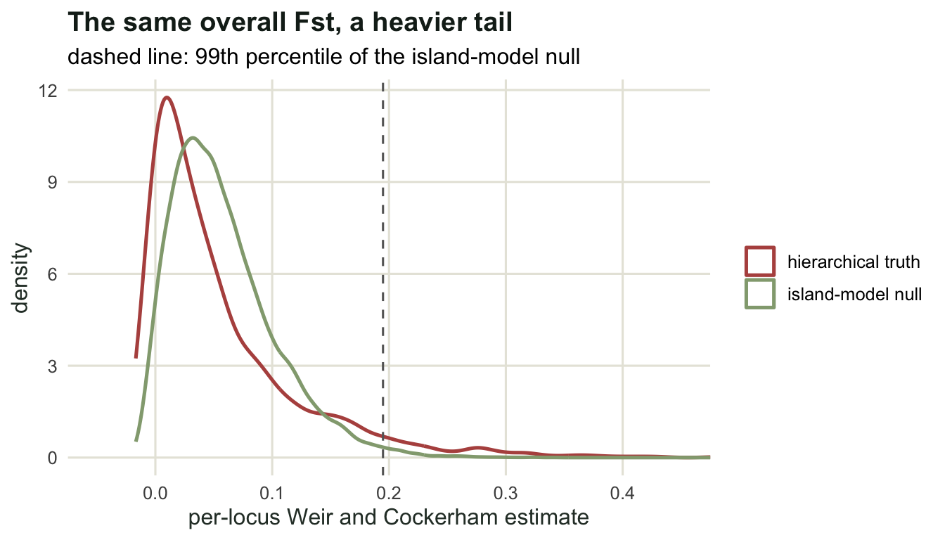
The fix is a null that matches the sampling: a hierarchical island model with the groups declared, or a demographic model fitted to the data first, or a scan that conditions on the observed covariance among populations. None of these is a formality. An outlier scan is a comparison against a model of the population’s history, so it answers “is this locus unusual given that history”, and if the history is wrong the answer is about the history.
The honest limit
The four checks constrain a population genetic analysis; they do not validate it. Two things they cannot reach are worth stating plainly.
The first is that no property of allele frequencies separates selection from demography at a single locus. A bottleneck, a range expansion, or an unsampled ghost population all produce loci with extreme Fst, and they do it without any locus being special. The evidence that promotes a candidate from a list to a result comes from outside the scan: a repeated signal in an independent population pair, a match to an environmental gradient, a function that makes sense, an experiment.
The second is that all four checks assume the marker set is a fair sample of the genome. Markers chosen because they were variable in one population, or an assay developed on one lineage, tilt every statistic in this cluster in the same direction, and no internal diagnostic can see it, because the data set does not contain the loci that were never assayed. That is the same shape of problem as the omitted trait in a selection analysis: the fix is in the design, not in the diagnostics.
Where to go next
That closes the population genetics cluster: expectations for one locus in one population, F-statistics for many populations, the drift and migration processes that predict Fst, and the checks. The natural continuation is the other place where allele frequencies change on their own, the stochastic dynamics of finite populations, where the same binomial sampling that produced drift here drives fixation probabilities and evolutionary outcomes.
References
Weir BS, Cockerham CC 1984 Evolution 38(6):1358-1370 (10.1111/j.1558-5646.1984.tb05657.x)
Beaumont MA, Nichols RA 1996 Proceedings of the Royal Society B 263(1377):1619-1626 (10.1098/rspb.1996.0237)
Excoffier L, Hofer T, Foll M 2009 Heredity 103(4):285-298 (10.1038/hdy.2009.74)
Willing EM, Dreyer C, van Oosterhout C 2012 PLoS ONE 7(8):e42649 (10.1371/journal.pone.0042649)
Lotterhos KE, Whitlock MC 2014 Molecular Ecology 23(9):2178-2192 (10.1111/mec.12725)
Bhatia G, Patterson N, Sankararaman S, Price AL 2013 Genome Research 23(9):1514-1521 (10.1101/gr.154831.113)
Dakin EE, Avise JC 2004 Heredity 93(5):504-509 (10.1038/sj.hdy.6800545)