Drift, migration and isolation by distance

Simulate drift and gene flow in R, check the Fst equilibrium against 1/(1 + 4Nm), and see how little a measured Fst says about the number of migrants.

Fst earns its place in ecology because theory predicts it. Two forces set it: drift pushes populations apart at a rate governed by their size, gene flow pulls them back together. Balance the two and you get the most quoted equation in the field, Fst = 1/(1 + 4Nm), which appears to convert a genetic measurement into a number of migrants per generation.

This tutorial builds both halves of that balance from scratch, confirms the equilibrium against simulation, and then works out what the equation licenses you to say. The short answer is: much less than it looks, and the reasons are worth knowing before a reviewer supplies them.

Drift alone

A Wright-Fisher deme of N diploids passes 2N gene copies to the next generation by binomial sampling. Nothing here is directional; the allele frequency simply wanders. Start 2000 isolated demes at the same frequency and watch them spread apart.

library(ggplot2)

te_pal <- list(forest = "#275139", green = "#2f8f63", sage = "#93a87f",
               clay = "#b5534e", gold = "#cda23f", line = "#dad9ca",
               ink = "#16241d")

theme_te <- function() {
  theme_minimal(base_size = 12) +
    theme(panel.grid.minor = element_blank(),
          panel.grid.major = element_line(colour = "#e7e6dc"),
          plot.background = element_rect(fill = "white", colour = NA),
          panel.background = element_rect(fill = "white", colour = NA),
          plot.title = element_text(face = "bold", colour = te_pal$ink),
          axis.title = element_text(colour = "#2c3a31"))
}

set.seed(466)

n_dip <- 25
n_demes <- 2000
gens <- 60

p_mat <- matrix(NA_real_, gens + 1, n_demes)
p_mat[1, ] <- 0.5
for (g in seq_len(gens)) {
  p_mat[g + 1, ] <- rbinom(n_demes, 2 * n_dip, p_mat[g, ]) / (2 * n_dip)
}

fst_sim <- apply(p_mat, 1, function(p) {
  p_bar <- mean(p)
  mean((p - p_bar)^2) / (p_bar * (1 - p_bar))
})
fst_pred <- 1 - (1 - 1 / (2 * n_dip))^(0:gens)

rows <- c(1, 11, 26, 51, 61)
print(round(data.frame(generation = (0:gens)[rows],
                       simulated = fst_sim[rows],
                       predicted = fst_pred[rows]), 4))

  generation simulated predicted
1          0    0.0000    0.0000
2         10    0.1879    0.1829
3         25    0.3995    0.3965
4         50    0.6337    0.6358
5         60    0.6938    0.7024

cat("demes fixed for one allele by generation 60:",
    round(mean(p_mat[gens + 1, ] %in% c(0, 1)), 4),
    " mean allele frequency:", round(mean(p_mat[gens + 1, ]), 4), "\n")

demes fixed for one allele by generation 60: 0.5595  mean allele frequency: 0.5063 

The variance among demes grows on a clock ticking at 1/(2N) per generation, so Fst after t generations is 1 - (1 - 1/(2N))^t. Simulation gives 0.1879 at generation 10 against a predicted 0.1829, and 0.6337 at generation 50 against 0.6358. The mean allele frequency has not moved (0.5063): drift does not push in a direction, it only spreads.

The second line of output is the part that matters for conservation work. By generation 60, 55.95 percent of the demes have lost one allele entirely. Small isolated populations do not drift towards being different, they drift towards being monomorphic, and the differentiation is a byproduct of that loss.

drift_df <- data.frame(generation = 0:gens, simulated = fst_sim,
                       predicted = fst_pred)
ggplot(drift_df, aes(generation)) +
  geom_line(aes(y = predicted), linetype = "dashed", colour = "grey50",
            linewidth = 0.8) +
  geom_line(aes(y = simulated), colour = te_pal$forest, linewidth = 0.9) +
  labs(title = "Isolated demes drift apart on a clock set by N",
       subtitle = "solid: 2000 simulated demes of 25 diploids, dashed: 1 - (1 - 1/(2N))^t",
       x = "generation", y = "Fst") +
  theme_te()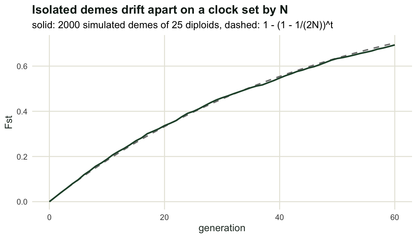

Figure 1: Fst among 2000 isolated demes of 25 diploids, simulated against the prediction 1 - (1 - 1/(2N))^t.

Adding gene flow

Now let a fraction m of each deme be replaced every generation by immigrants drawn from a common pool. Migration pulls every deme back towards the pool frequency, drift pushes it away, and the two settle into a stationary distribution rather than a fixed value. Under the island model that distribution is a beta, and its variance gives the classic result.

island_fst <- function(n_dip, m, n_demes = 2000, burn = 3000, keep = 500,
                       p_pool = 0.5) {
  p <- rep(p_pool, n_demes)
  acc <- numeric(keep)
  for (g in seq_len(burn + keep)) {
    p_mig <- (1 - m) * p + m * p_pool
    p <- rbinom(n_demes, 2 * n_dip, p_mig) / (2 * n_dip)
    if (g > burn) {
      acc[g - burn] <- mean((p - p_pool)^2) / (p_pool * (1 - p_pool))
    }
  }
  mean(acc)
}

set.seed(467)
m_grid <- c(0.001, 0.005, 0.01, 0.05, 0.1)
isl <- data.frame(m = m_grid, Nm = 50 * m_grid,
                  simulated = sapply(m_grid, function(m) island_fst(50, m)),
                  predicted = 1 / (1 + 4 * 50 * m_grid))
print(round(isl, 4))

      m   Nm simulated predicted
1 0.001 0.05    0.8314    0.8333
2 0.005 0.25    0.5047    0.5000
3 0.010 0.50    0.3403    0.3333
4 0.050 2.50    0.0940    0.0909
5 0.100 5.00    0.0505    0.0476

Five migration rates, 50 diploids per deme, and the simulated stationary Fst lands on 1/(1 + 4Nm) every time: 0.8314 against 0.8333, 0.3403 against 0.3333, 0.0505 against 0.0476. The residual is the price of a continuous approximation applied to a discrete binomial process, and it grows slightly with m, which is the regime where the approximation is weakest.

Look at the second column rather than the first. What controls Fst is Nm, the number of migrant individuals per generation, not the migration rate. Half a migrant per generation gives Fst = 0.33; five migrants give 0.05. A population of 50 exchanging one percent of itself and a population of 5000 exchanging one hundredth of one percent have the same expected Fst, and the same conclusion follows for both.

curve_df <- data.frame(Nm = 10^seq(log10(0.04), log10(6), length.out = 200))
curve_df$fst <- 1 / (1 + 4 * curve_df$Nm)

ggplot(curve_df, aes(Nm, fst)) +
  geom_line(colour = te_pal$sage, linewidth = 1.1) +
  geom_point(data = isl, aes(Nm, simulated), colour = te_pal$forest,
             size = 2.6) +
  scale_x_log10() +
  labs(title = "One migrant per generation is the hinge",
       subtitle = "line: 1/(1 + 4Nm), points: simulated island model, N = 50",
       x = "migrants per generation Nm (log scale)",
       y = "stationary Fst") +
  theme_te()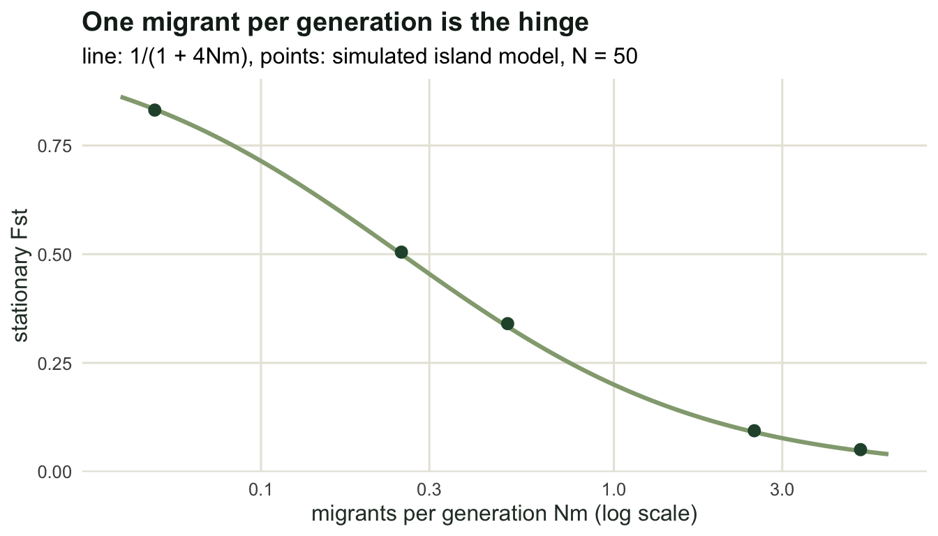

Figure 2: Stationary Fst against the number of migrants per generation. Points are simulated island models with 50 diploids per deme; the line is 1/(1 + 4Nm).

How long does an Fst remember?

An equilibrium is a promise about the far future. Real populations were connected differently a century ago, so it matters how quickly Fst forgets. Start every deme at the pool frequency, which is Fst = 0, and time the approach.

set.seed(468)

approach <- function(n_dip, m, n_demes = 4000, gens = 200, p_pool = 0.5) {
  p <- rep(p_pool, n_demes)
  out <- numeric(gens)
  for (g in seq_len(gens)) {
    p <- rbinom(n_demes, 2 * n_dip, (1 - m) * p + m * p_pool) / (2 * n_dip)
    out[g] <- mean((p - p_pool)^2) / (p_pool * (1 - p_pool))
  }
  out
}

app <- approach(50, 0.01)
eq <- 1 / (1 + 4 * 50 * 0.01)
cat("equilibrium Fst:", round(eq, 4),
    " generations to half of it:", which(app >= eq / 2)[1],
    " to 90 percent of it:", which(app >= 0.9 * eq)[1], "\n")

equilibrium Fst: 0.3333  generations to half of it: 23  to 90 percent of it: 72 

cat("Fst at generations 10, 25, 50, 100 and 200:",
    round(app[c(10, 25, 50, 100, 200)], 4), "\n")

Fst at generations 10, 25, 50, 100 and 200: 0.0894 0.1833 0.2589 0.3231 0.3457 

With N = 50 and m = 0.01 the equilibrium is 0.3333, half of it arrives in 23 generations and 90 percent of it in 72. That is fast, and it is fast because the relevant timescale is set by whichever is quicker, migration at rate 2m or drift at rate 1/(2N). Make the populations larger or the migration weaker and the memory lengthens, in proportion. A large, weakly connected system can carry the signature of a landscape that no longer exists, and there is no way to tell from the Fst value alone: it is a single number, and the number of generations since the connection changed is not in it.

Inverting the equation

Rearranged, Nm = (1 - Fst)/(4 Fst). The temptation is obvious and so is the problem.

fst_vals <- c(0.01, 0.02, 0.03, 0.05, 0.1, 0.2)
print(round(data.frame(Fst = fst_vals,
                       Nm = (1 - fst_vals) / (4 * fst_vals)), 3))

   Fst     Nm
1 0.01 24.750
2 0.02 12.250
3 0.03  8.083
4 0.05  4.750
5 0.10  2.250
6 0.20  1.000

At the low end, where most outbred species sit, the inversion is nearly vertical. An Fst of 0.02 implies 12.25 migrants per generation and an Fst of 0.03 implies 8.08: a shift of 0.01 in a quantity that scatters more than that from locus to locus moves the answer by four migrants. Estimate Fst badly, or from few loci, and the migration estimate is decoration.

The deeper problem is that Nm is a product. Nothing in the genetic data separates N from m, so a value of Nm = 1 is equally consistent with 10 individuals exchanging 10 percent and 1000 individuals exchanging one tenth of one percent, which are different situations for a manager. Add the assumptions the island model makes, and Whitlock and McCauley’s list is long: equal deme sizes, symmetric migration, no extinction and recolonisation, no selection, and equilibrium reached. Every one of them fails somewhere in a real landscape, and they do not fail conservatively.

The defensible use of Fst is comparative. Is this population pair more differentiated than that one, does differentiation track distance or a barrier, has it changed between two sampling periods. Those questions need Fst to be a consistent measurement, not an unbiased estimate of a migration rate.

Isolation by distance

Comparative use has one classic form. If dispersal is local rather than global, differentiation should grow with geographic distance, and the growth carries information about how local dispersal is. Simulate a line of 30 demes exchanging migrants only with their neighbours, with a small mutation rate so that variation is not eventually lost, and 200 independent loci so the pairwise estimates are not pure noise.

step_stone <- function(n_deme = 30, n_dip = 50, m = 0.05, u = 1e-4,
                       n_loci = 200, gens = 3000) {
  mig <- diag(n_deme) * (1 - m)
  for (i in seq_len(n_deme)) {
    left <- if (i == 1) i else i - 1
    right <- if (i == n_deme) i else i + 1
    mig[i, left] <- mig[i, left] + m / 2
    mig[i, right] <- mig[i, right] + m / 2
  }
  p <- matrix(0.5, n_loci, n_deme)
  for (g in seq_len(gens)) {
    p <- p %*% t(mig)
    p <- p * (1 - u) + (1 - p) * u
    p <- matrix(rbinom(length(p), 2 * n_dip, as.vector(p)),
                nrow = n_loci) / (2 * n_dip)
  }
  p
}

pair_fst <- function(p) {
  n_deme <- ncol(p)
  res <- NULL
  for (i in 1:(n_deme - 1)) {
    for (j in (i + 1):n_deme) {
      p_bar <- (p[, i] + p[, j]) / 2
      hs <- (2 * p[, i] * (1 - p[, i]) + 2 * p[, j] * (1 - p[, j])) / 2
      ht <- 2 * p_bar * (1 - p_bar)
      res <- rbind(res, data.frame(dist = j - i, num = sum(ht - hs),
                                   den = sum(ht)))
    }
  }
  agg <- aggregate(cbind(num, den) ~ dist, res, sum)
  agg$fst <- agg$num / agg$den
  agg$lin <- agg$fst / (1 - agg$fst)
  agg
}

set.seed(469)
agg <- pair_fst(step_stone())
print(round(agg[agg$dist %in% c(1, 2, 5, 10, 15, 20, 29),
                c("dist", "fst", "lin")], 4))

   dist    fst    lin
1     1 0.0466 0.0488
2     2 0.0850 0.0929
5     5 0.1773 0.2154
10   10 0.2723 0.3741
15   15 0.3355 0.5049
20   20 0.3931 0.6478
29   29 0.5385 1.1670

fit <- lm(lin ~ dist, data = subset(agg, dist <= 15))
cat("slope over distances 1 to 15:", round(coef(fit)[[2]], 5),
    " intercept:", round(coef(fit)[[1]], 5),
    " r squared:", round(summary(fit)$r.squared, 4), "\n")

slope over distances 1 to 15: 0.0319  intercept: 0.04467  r squared: 0.9901 

Neighbouring demes sit at Fst = 0.0466 and demes 29 steps apart at 0.5385, from a model with no barriers and no selection: the pattern is produced by distance alone. Following Rousset, the quantity that should be linear in distance is Fst/(1 - Fst), and over distances 1 to 15 it is, with an r squared of 0.9901 and a slope of 0.0319.

ggplot(agg, aes(dist, lin)) +
  geom_abline(intercept = coef(fit)[[1]], slope = coef(fit)[[2]],
              colour = te_pal$clay, linewidth = 0.9) +
  geom_point(colour = te_pal$forest, size = 2) +
  labs(title = "Differentiation grows with distance, with nothing driving it",
       subtitle = "30 demes in a line, N = 50, m = 0.05, 200 loci, fit over distances 1 to 15",
       x = "distance in demes", y = "Fst / (1 - Fst)") +
  theme_te()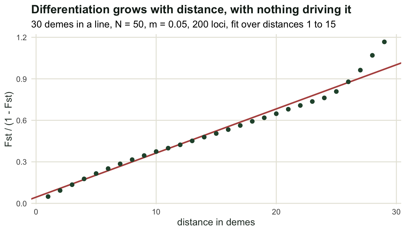

Figure 3: Linearised pairwise Fst against distance along a 30-deme stepping stone, with the regression fitted over distances 1 to 15.

The slope is where the interpretation happens, because theory relates it to 1/(4 N sigma^2), with sigma^2 the mean squared parent-offspring displacement. Repeating the simulation over deme sizes and migration rates tests that relation directly.

set.seed(470)
cfg <- data.frame(n_dip = c(50, 100, 50, 25), m = c(0.05, 0.05, 0.10, 0.05))
cfg$slope <- NA_real_
for (k in seq_len(nrow(cfg))) {
  a_k <- pair_fst(step_stone(n_dip = cfg$n_dip[k], m = cfg$m[k]))
  cfg$slope[k] <- coef(lm(lin ~ dist, data = subset(a_k, dist <= 15)))[[2]]
}
cfg$naive_pred <- 1 / (4 * cfg$n_dip * cfg$m)
cfg$ratio <- cfg$slope / cfg$naive_pred
print(round(cfg, 4))

  n_dip    m  slope naive_pred  ratio
1    50 0.05 0.0308       0.10 0.3084
2   100 0.05 0.0156       0.05 0.3121
3    50 0.10 0.0198       0.05 0.3953
4    25 0.05 0.0674       0.20 0.3370

cat("slope ratio when deme size doubles:",
    round(cfg$slope[1] / cfg$slope[2], 3),
    " when migration doubles:", round(cfg$slope[1] / cfg$slope[3], 3), "\n")

slope ratio when deme size doubles: 1.976  when migration doubles: 1.56 

Doubling deme size from 50 to 100 halves the slope, 0.0308 to 0.0156, exactly as 1/(4 N sigma^2) requires. The migration rate behaves less cleanly: doubling m from 0.05 to 0.10 divides the slope by 1.50 rather than by 2, because the identity sigma^2 = m only holds while m is small. And in every row the measured slope is roughly a third of the naive prediction (ratios 0.31, 0.31, 0.41 and 0.33), because the derivation assumes an unbounded lattice while this one has 30 demes and two edges.

That gap is the honest limit of isolation by distance analysis. The shape of the relation is real and reliable: local dispersal produces a linear rise of Fst/(1 - Fst) with distance, and a steeper slope does mean more restricted gene flow. Converting a slope into a neighbourhood size or a dispersal variance needs a model that matches the sampled landscape in shape, extent and dispersal kernel, and the constant of proportionality is the thing that moves when the model is wrong. Report the slope and compare slopes; be careful with the metres.

Where to go next

Three tutorials in, every number here has come from data with a known answer, which is a luxury real projects do not have. The last tutorial in this cluster is about the checks that survive that transition: how many loci and how many individuals a usable Fst needs, how to tell a marker problem from a biological one, what filtering rare variants does to the answer, and why an outlier test for selection needs a demographic null before it means anything.

References

Wright S 1931 Genetics 16(2):97-159 (10.1093/genetics/16.2.97)

Wright S 1943 Genetics 28(2):114-138 (10.1093/genetics/28.2.114)

Kimura M, Weiss GH 1964 Genetics 49(4):561-576 (10.1093/genetics/49.4.561)

Slatkin M 1993 Evolution 47(1):264-279 (10.1111/j.1558-5646.1993.tb01215.x)

Rousset F 1997 Genetics 145(4):1219-1228 (10.1093/genetics/145.4.1219)

Whitlock MC, McCauley DE 1999 Heredity 82(2):117-125 (10.1038/sj.hdy.6884960)

Related tutorials

• Hardy-Weinberg expectations
• F-statistics and population structure
• Checking a population genetics analysis
• The Moran process and fixation probability