library(ggplot2)
library(patchwork)

te_paper  <- "#f5f4ee"
te_ink    <- "#16241d"
te_body   <- "#2c3a31"
te_forest <- "#275139"
te_rust   <- "#b5534e"
te_gold   <- "#c9b458"
te_line   <- "#dad9ca"

theme_datasheet <- function() {
  theme_minimal(base_size = 12) +
    theme(plot.background  = element_rect(fill = te_paper, colour = NA),
          panel.background = element_rect(fill = te_paper, colour = NA),
          panel.grid.major = element_line(colour = te_line, linewidth = 0.3),
          panel.grid.minor = element_blank(),
          text             = element_text(colour = te_body),
          plot.title       = element_text(colour = te_ink, face = "bold"),
          plot.subtitle    = element_text(colour = te_body),
          axis.text        = element_text(colour = te_body))
}Detecting sex-biased dispersal from genotypes
R
population genetics
dispersal
permutation test
simulation
ecology tutorial
Testing sex-biased dispersal in R with Fst and assignment indices: calibrated permutation tests and why power is signal over noise, not immigrant counts.
A shrew population is trapped in sixteen hedgerow patches, a dozen adult females and a dozen adult males in each, and every animal gets an ear clip and a panel of sixty SNPs. The field team has watched juveniles leave in spring and has an impression that it is mostly the young females that go. Nobody can follow enough of them to put a number on it. The genotypes are already in the freezer, and the question is whether they can say which sex moves.
They can, in principle. An adult that was born in another patch carries a genotype drawn from that patch’s allele frequencies, so a sample from the more dispersive sex holds more of these outsiders. Its allele frequencies look less like the patch it was caught in, its differentiation among patches is lower, and its members fit their own patch less well on average. Favre and colleagues used the assignment version of this idea on the greater white-toothed shrew, Goudet, Perrin and Waser compared several such statistics as permutation tests on biparentally inherited markers, and Prugnolle and de Meeus reviewed the genetic approaches to sex-biased dispersal. The catch is built into the logic: the signal exists only in a narrow window of the life cycle, after the juveniles have dispersed and before the immigrants breed and mix their genes into the local pool.
On this site gene flow has so far been a single number per deme. Drift, migration and isolation by distance replaces a fraction m of each deme with immigrants every generation and checks the equilibrium Fst against 1/(1 + 4Nm), with no sexes anywhere in the model. F-statistics and population structure builds the Weir and Cockerham estimator from its variance components and shows why a small sample needs it; that estimator is reused here, once for each sex. Assignment tests and self-assignment scores genotypes against baseline populations to find where an individual came from. Here nobody is assigned to a source. The genotype likelihood is used only to ask whether one sex, as a group, fits its home patch worse than the other.
The post builds the island model with separate dispersal rates for the two sexes, checks its short burn-in against an individual based version, runs three sex-bias statistics with a within-patch permutation of sex labels, and then measures calibration and power over a grid of bias and total dispersal. An obvious guess is that power follows the number of immigrants in the sample. The measurement agrees only roughly, and the reason turns out to be simple arithmetic: power is the size of the signal against the noise, and the immigrant count mixes the two.
An island model with two dispersal rates
The metapopulation has sixteen demes of one hundred adults, half of each sex. Each generation the adults breed at random within their deme and the juveniles disperse, a female with probability d_f and a male with probability d_m, to a deme chosen at random among the other fifteen. For autosomal genes what matters over many generations is the mean of the two rates, because every juvenile has one mother and one father; the difference between the rates only matters in the one generation that is sampled.
n_deme    <- 16      # demes (patches)
n_adult   <- 100     # adults per deme, half of each sex
n_sex     <- 12      # adults of each sex sampled per deme
n_loci    <- 60      # biallelic SNPs
n_perm    <- 99      # permutations of sex labels per test
alpha_lev <- 0.05    # one sided, female-biased dispersal as the alternative

# frequency-level burn-in at the mean dispersal rate, run for five relaxation
# times of the island model; returns an array replicate x locus x deme
burn_freq <- function(n_rep, n_loc, d_bar) {
  n_gen <- ceiling(5 / (2 * d_bar + 1 / (2 * n_adult)))
  p <- matrix(rep(runif(n_rep * n_loc, 0.1, 0.9), n_deme), ncol = n_deme)
  for (g in seq_len(n_gen)) {
    tot  <- rowSums(p)
    p_in <- (1 - d_bar) * p + d_bar * (tot - p) / (n_deme - 1)
    p[]  <- rbinom(length(p), 2 * n_adult, p_in) / (2 * n_adult)
  }
  array(p, c(n_rep, n_loc, n_deme))
}

ratio_fst <- function(p) {          # parametric Fst of true deme frequencies
  p_bar <- rowMeans(p)
  sum(rowSums((p - p_bar)^2) / (ncol(p) - 1)) / sum(p_bar * (1 - p_bar))
}
Tracking allele frequencies instead of individuals makes the burn-in cheap, but it is a shortcut that has to be checked. The individual based version below keeps every genotype, gives each juvenile a mother and a father from its natal deme, moves females and males at their own rates, and records the realised Fst of the adults over two hundred generations after a burn-in of fifty.
ind_sim <- function(n_loc, d_f, d_m, n_gen, keep) {
  n_tot <- n_deme * n_adult
  deme  <- rep(seq_len(n_deme), each = n_adult)
  fem   <- rep(rep(c(TRUE, FALSE), each = n_adult / 2), n_deme)
  p0    <- runif(n_loc, 0.1, 0.9)
  geno  <- matrix(rbinom(n_tot * n_loc, 2, rep(p0, each = n_tot)), n_tot)
  fst_trace <- numeric(0)
  for (g in seq_len(n_gen)) {
    mover <- runif(n_tot) < ifelse(fem, d_f, d_m)
    natal <- ifelse(mover, (deme - 1 + sample.int(n_deme - 1, n_tot, TRUE)) %% n_deme + 1, deme)
    mum <- (natal - 1) * n_adult + sample.int(n_adult / 2, n_tot, TRUE)
    dad <- (natal - 1) * n_adult + n_adult / 2 + sample.int(n_adult / 2, n_tot, TRUE)
    geno <- matrix(rbinom(n_tot * n_loc, 1, geno[mum, ] / 2) +
                   rbinom(n_tot * n_loc, 1, geno[dad, ] / 2), n_tot)
    if (g > n_gen - keep)
      fst_trace <- c(fst_trace, ratio_fst(t(rowsum(geno, deme)) / (2 * n_adult)))
  }
  fst_trace
}

d_chk <- c(f = 0.15, m = 0.05)
set.seed(4101)
trace_ind <- ind_sim(n_loci, d_chk[["f"]], d_chk[["m"]], n_gen = 250, keep = 200)
fst_ind   <- mean(trace_ind)
se_ind    <- sd(colMeans(matrix(trace_ind, nrow = 20))) / sqrt(10)   # ten blocks of 20
set.seed(4102)
fst_freq  <- ratio_fst(matrix(burn_freq(400, n_loci, mean(d_chk)), ncol = n_deme))
fst_eq    <- 1 / (1 + 4 * n_adult * mean(d_chk))
With d_f = 0.15 and d_m = 0.05, the individual based model settles at an Fst of 0.0242 (block standard error 0.0003). The frequency-level burn-in at the mean rate gives 0.0243, and the island formula 1/(1 + 4Nm) with the mean rate gives 0.0244. The shortcut reproduces the individual model, and the sex difference in dispersal leaves no trace in the adult Fst of the whole population.
Sampling after dispersal
The sample is taken from adults who have dispersed and not yet bred. Each sampled animal is an immigrant with the probability for its sex, and an immigrant’s genotype is drawn from the allele frequencies of the deme it was born in. The second option in the function samples the next stage instead: the adults, including their immigrants, breed, and a dozen offspring of each sex are genotyped before they disperse.
sample_study <- function(p, d_f, d_m, n_per = n_sex, stage = "adults") {
  n_loc <- nrow(p)
  draw <- function(n_each) {
    deme  <- rep(seq_len(n_deme), each = 2 * n_each)
    fem   <- rep(rep(c(TRUE, FALSE), each = n_each), n_deme)
    imm   <- runif(length(deme)) < ifelse(fem, d_f, d_m)
    natal <- ifelse(imm, (deme - 1 + sample.int(n_deme - 1, length(deme), TRUE)) %% n_deme + 1, deme)
    geno  <- matrix(rbinom(length(deme) * n_loc, 2, t(p[, natal])), nrow = length(deme))
    list(geno = geno, deme = deme, fem = fem, imm = imm)
  }
  if (stage == "adults") return(draw(n_per))
  adults <- draw(n_adult / 2)                       # whole post-dispersal deme
  p_now  <- t(rowsum(adults$geno, adults$deme)) / (2 * n_adult)
  kids   <- draw(n_per)
  kids$geno <- matrix(rbinom(length(kids$deme) * n_loc, 2, t(p_now[, kids$deme])),
                      nrow = length(kids$deme))
  kids$imm[] <- FALSE
  kids
}
Three statistics and one permutation
Three statistics are computed for each study. The first is the Weir and Cockerham theta across the sixteen demes, estimated separately from the females and from the males (multilocus: the sum of the among-deme components over loci divided by the sum of all components). The dispersing sex should have the lower value. The other two use the corrected assignment index of Favre and colleagues. For each animal the log10 probability of its genotype is computed under Hardy-Weinberg proportions with the allele frequencies of the deme it was caught in, estimated from both sexes and including the animal itself; subtracting the deme mean gives the corrected index AIc, which averages zero in every deme. Immigrants tend to have negative values, so the dispersing sex should have a lower mean (mAIc) and a larger variance (vAIc).
The null distribution comes from shuffling the sex labels among the animals of each deme, which keeps twelve of each sex per deme and leaves every genotype where it was caught. Each test is one sided in the direction of female-biased dispersal, fixed before any simulation was run, and the p value counts the observed statistic among its 99 permutations.
wc_theta_arr <- function(x, h, n, r) {       # x, h: permutation x locus x deme
  pp <- x / (2 * n); hw <- rowMeans(h, dims = 2) / n
  pw <- rowMeans(pp, dims = 2)
  s2 <- (rowSums(pp^2, dims = 2) - r * pw^2) / (r - 1)
  pq <- pw * (1 - pw)
  a_comp <- s2 - (pq - (r - 1) / r * s2 - hw / 4) / (n - 1)
  b_comp <- n / (n - 1) * (pq - (r - 1) / r * s2 - (2 * n - 1) / (4 * n) * hw)
  rowSums(a_comp) / rowSums(a_comp + b_comp + hw / 2)
}

sbd_test <- function(st, n_pm = n_perm) {
  geno <- st$geno + 0; r <- n_deme; n_ind <- nrow(geno); n <- n_ind / r / 2
  het  <- (geno == 1) * 1
  # sex labels shuffled within deme: row 1 is the observed labelling
  u_mat <- matrix(runif(n_pm * n_ind), n_pm)
  key   <- (row(u_mat) - 1) * r + rep(st$deme - 1, each = n_pm) + u_mat
  lab   <- matrix(0, n_pm, n_ind)
  lab[order(key)] <- rep(rep(c(1, 0), each = n), r * n_pm)
  lab   <- rbind(st$fem * 1, lab)
  # corrected assignment index
  cnt  <- rowsum(geno, st$deme, reorder = TRUE)
  p_d  <- pmin(pmax(cnt / (4 * n), 1e-12), 1 - 1e-12)
  ai   <- rowSums(geno * log10(p_d)[st$deme, ] + (2 - geno) * log10(1 - p_d)[st$deme, ]) +
          log10(2) * rowSums(het)
  aic  <- ai - ave(ai, st$deme)
  # Weir and Cockerham theta for each sex under every labelling
  hcnt <- rowsum(het, st$deme, reorder = TRUE)
  x_f <- vapply(seq_len(r), function(d) {
    idx <- which(st$deme == d); lab[, idx] %*% geno[idx, ] }, matrix(0, n_pm + 1, ncol(geno)))
  h_f <- vapply(seq_len(r), function(d) {
    idx <- which(st$deme == d); lab[, idx] %*% het[idx, ] }, matrix(0, n_pm + 1, ncol(geno)))
  fst_f <- wc_theta_arr(x_f, h_f, n, r)
  fst_m <- wc_theta_arr(rep(t(cnt), each = n_pm + 1) - x_f,
                        rep(t(hcnt), each = n_pm + 1) - h_f, n, r)
  n_f <- n * r
  mean_f <- as.vector(lab %*% aic) / n_f
  mean_m <- -mean_f                                # AIc sums to zero in each deme
  ss_f   <- as.vector(lab %*% aic^2)
  var_f  <- (ss_f - n_f * mean_f^2) / (n_f - 1)
  var_m  <- (sum(aic^2) - ss_f - n_f * mean_m^2) / (n_f - 1)
  stat <- cbind(fst = fst_m - fst_f, maic = mean_m - mean_f, vaic = var_f - var_m)
  p_val <- colMeans(stat >= rep(stat[1, ], each = n_pm + 1))
  c(p_val, fst_f = fst_f[1], fst_m = fst_m[1], gap = unname(stat[1, "fst"]),
    null_sd = sd(stat[-1, "fst"]), aic_f = mean_f[1],
    imm_f = sum(st$imm & st$fem), imm_m = sum(st$imm & !st$fem))
}

set.seed(4103)
p_one  <- burn_freq(1, n_loci, mean(d_chk))[1, , ]
study1 <- sample_study(p_one, d_chk[["f"]], d_chk[["m"]])
test1  <- sbd_test(study1)
In one simulated study at the same rates (the first draw from its seed), 29 of the 192 sampled females and 10 of the males were born elsewhere. Even so, female theta is 0.0183 against 0.0141 for males, the wrong way round, and the mean AIc of females is +0.031, above the male mean. The one sided p values are 0.85 for Fst, 0.69 for mAIc and 0.09 for vAIc. A threefold difference in dispersal, and this study sees none of it.
aic_all <- {
  geno <- study1$geno
  cnt  <- rowsum(geno, study1$deme, reorder = TRUE)
  p_d  <- pmin(pmax(cnt / (4 * n_sex), 1e-12), 1 - 1e-12)
  ai   <- rowSums(geno * log10(p_d)[study1$deme, ] + (2 - geno) * log10(1 - p_d)[study1$deme, ]) +
          log10(2) * rowSums(geno == 1)
  ai - ave(ai, study1$deme)
}
imm_mean <- mean(aic_all[study1$imm]); res_mean <- mean(aic_all[!study1$imm])
imm_below <- mean(aic_all[study1$imm] < 0); res_below <- mean(aic_all[!study1$imm] < 0)
aic_df <- data.frame(aic = aic_all,
                     sex = ifelse(study1$fem, "females", "males"),
                     origin = ifelse(study1$imm, "born in another deme", "born locally"))
ggplot(aic_df, aes(sex, aic)) +
  geom_hline(yintercept = 0, colour = te_body, linewidth = 0.4) +
  geom_jitter(aes(colour = origin, size = origin), width = 0.25, height = 0, alpha = 0.8) +
  stat_summary(fun = mean, geom = "crossbar", width = 0.6, linewidth = 0.5, colour = te_ink) +
  scale_colour_manual(values = c(`born in another deme` = te_rust, `born locally` = te_forest), name = NULL) +
  scale_size_manual(values = c(`born in another deme` = 2.4, `born locally` = 1.2), name = NULL) +
  labs(x = NULL, y = "corrected assignment index (log10)",
       title = "Immigrants fit their capture deme worse",
       subtitle = "black bar: mean of the sex") +
  theme_datasheet() + theme(legend.position = "top")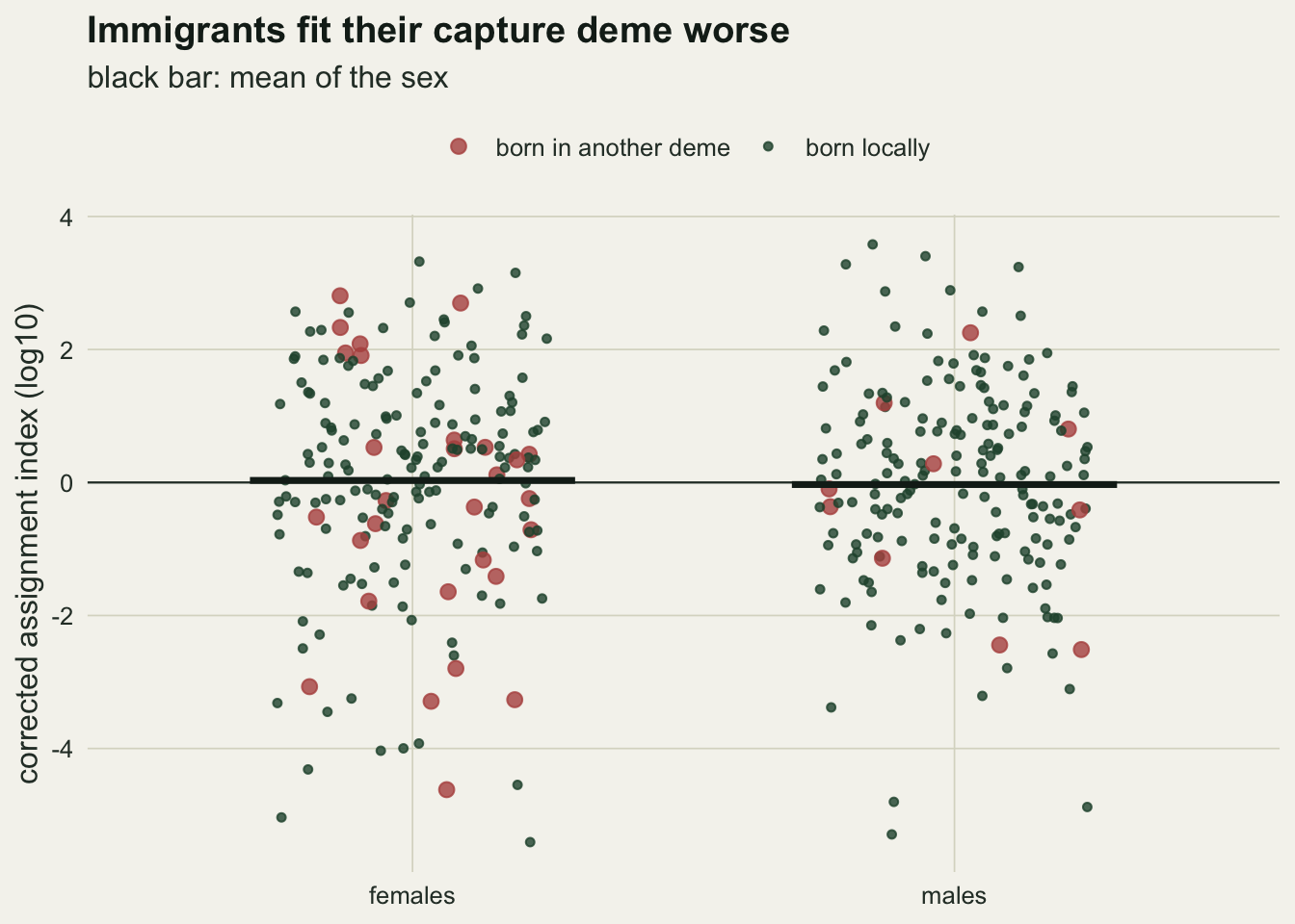
The plot shows the mechanism and also why it is weak. Immigrants average -0.31 against +0.04 for animals born locally, and 56 per cent of immigrants sit below zero against 45 per cent of residents. The two clouds overlap almost completely: at an Fst near 0.024 a genotype from another patch is only slightly less probable than a local one, sixty SNPs do not separate the groups, and the spread among residents is far wider than the shift that the immigrants add.
Calibration and power over a grid
The grid crosses three female to male dispersal ratios (1, 3 and 9) with three mean dispersal rates (0.02, 0.1 and 0.2). Ratio 1 is the null: both sexes move at the same rate, so the sex labels within a deme are exchangeable and a correct test rejects at its nominal rate. Replication was fixed before running: 200 studies per null cell and 400 per biased cell, each with its own burn-in.
run_cell <- function(n_rep, d_f, d_m, n_loc = n_loci, n_per = n_sex, stage = "adults") {
  p_all <- burn_freq(n_rep, n_loc, (d_f + d_m) / 2)
  out <- t(vapply(seq_len(n_rep), function(i)
    sbd_test(sample_study(p_all[i, , ], d_f, d_m, n_per, stage)), numeric(10)))
  attr(out, "f_adult") <- ratio_fst(matrix(p_all, ncol = n_deme))   # true adult Fst
  out
}
mcse <- function(p, n) sqrt(p * (1 - p) / n)

cells <- expand.grid(ratio = c(1, 3, 9), d_bar = c(0.02, 0.1, 0.2))
cells$d_f   <- 2 * cells$d_bar * cells$ratio / (1 + cells$ratio)
cells$d_m   <- 2 * cells$d_bar / (1 + cells$ratio)
cells$n_rep <- ifelse(cells$ratio == 1, 200, 400)

set.seed(4104)
grid_res <- lapply(seq_len(nrow(cells)), function(k)
  run_cell(cells$n_rep[k], cells$d_f[k], cells$d_m[k]))
for (s_nm in c("fst", "maic", "vaic"))
  cells[[paste0("pow_", s_nm)]] <- vapply(grid_res, function(x) mean(x[, s_nm] <= alpha_lev), 0)
cells$gap     <- vapply(grid_res, function(x) mean(x[, "gap"]), 0)
cells$null_sd <- vapply(grid_res, function(x) mean(x[, "null_sd"]), 0)
cells$fst_f   <- vapply(grid_res, function(x) mean(x[, "fst_f"]), 0)
cells$fst_m   <- vapply(grid_res, function(x) mean(x[, "fst_m"]), 0)

nul <- cells[cells$ratio == 1, ]
null_rates <- unlist(nul[, c("pow_fst", "pow_maic", "pow_vaic")])
se_null <- mcse(alpha_lev, 200)
pw <- function(ratio, d_bar, s_nm) cells[cells$ratio == ratio & cells$d_bar == d_bar, paste0("pow_", s_nm)]
se_max <- mcse(0.5, 400)
Under no bias the nine rejection rates (three statistics in three null cells) run from 0.025 to 0.055, against a nominal 0.05 and a Monte Carlo standard error of 0.015. The permutation of sex within demes is exact under exchangeability, and the simulation agrees.
With bias the three statistics do not behave alike. At a three-fold female bias the Fst test found it in 0.175, 0.287 and 0.280 of studies at mean dispersal 0.02, 0.1 and 0.2; at a nine-fold bias the same figures are 0.233, 0.525 and 0.595. The Monte Carlo standard error of a biased cell is at most 0.025, so the rise from the lowest dispersal is real at both ratios, while the three-fold values at 0.1 and 0.2 are too close to rank. Even the best cell misses the bias in 40 per cent of studies.
The mAIc test never beats the Fst test, with power between 0.110 and 0.230 and little change with dispersal. The vAIc test does the opposite of the Fst test: it is at its best at the lowest dispersal, 0.207 at a three-fold bias and 0.320 at nine-fold, higher than Fst in both cells (within Monte Carlo error at three-fold, clearly at nine-fold), and it falls to 0.055 and 0.100 at mean dispersal 0.2. Which statistic is the most powerful depends on how much dispersal there is, which is the thing the study does not know.
pow_long <- do.call(rbind, lapply(c("fst", "maic", "vaic"), function(s_nm) {
  data.frame(ratio = paste0("female:male ratio ", cells$ratio),
             d_bar = factor(cells$d_bar), n_rep = cells$n_rep,
             stat = c(fst = "Fst", maic = "mAIc", vaic = "vAIc")[[s_nm]],
             power = cells[[paste0("pow_", s_nm)]])
}))
pow_long$se <- mcse(pow_long$power, pow_long$n_rep)
power_plot <- function(dat) {
  ggplot(dat, aes(d_bar, power, colour = stat, group = stat)) +
    geom_hline(yintercept = alpha_lev, linetype = "dashed", colour = te_body) +
    geom_line(linewidth = 0.8, position = position_dodge(width = 0.3)) +
    geom_errorbar(aes(ymin = power - 2 * se, ymax = power + 2 * se), width = 0,
                  linewidth = 0.6, position = position_dodge(width = 0.3)) +
    geom_point(size = 2.2, position = position_dodge(width = 0.3)) +
    scale_colour_manual(values = c(Fst = te_forest, mAIc = te_gold, vAIc = te_rust), name = NULL) +
    scale_y_continuous(limits = c(0, 0.75)) +
    labs(x = "mean dispersal rate of the two sexes", y = "rejection rate") +
    theme_datasheet() + theme(legend.position = "top")
}
power_plot(pow_long) + facet_wrap(~ ratio) +
  labs(title = "Fst gains power with dispersal, vAIc loses it")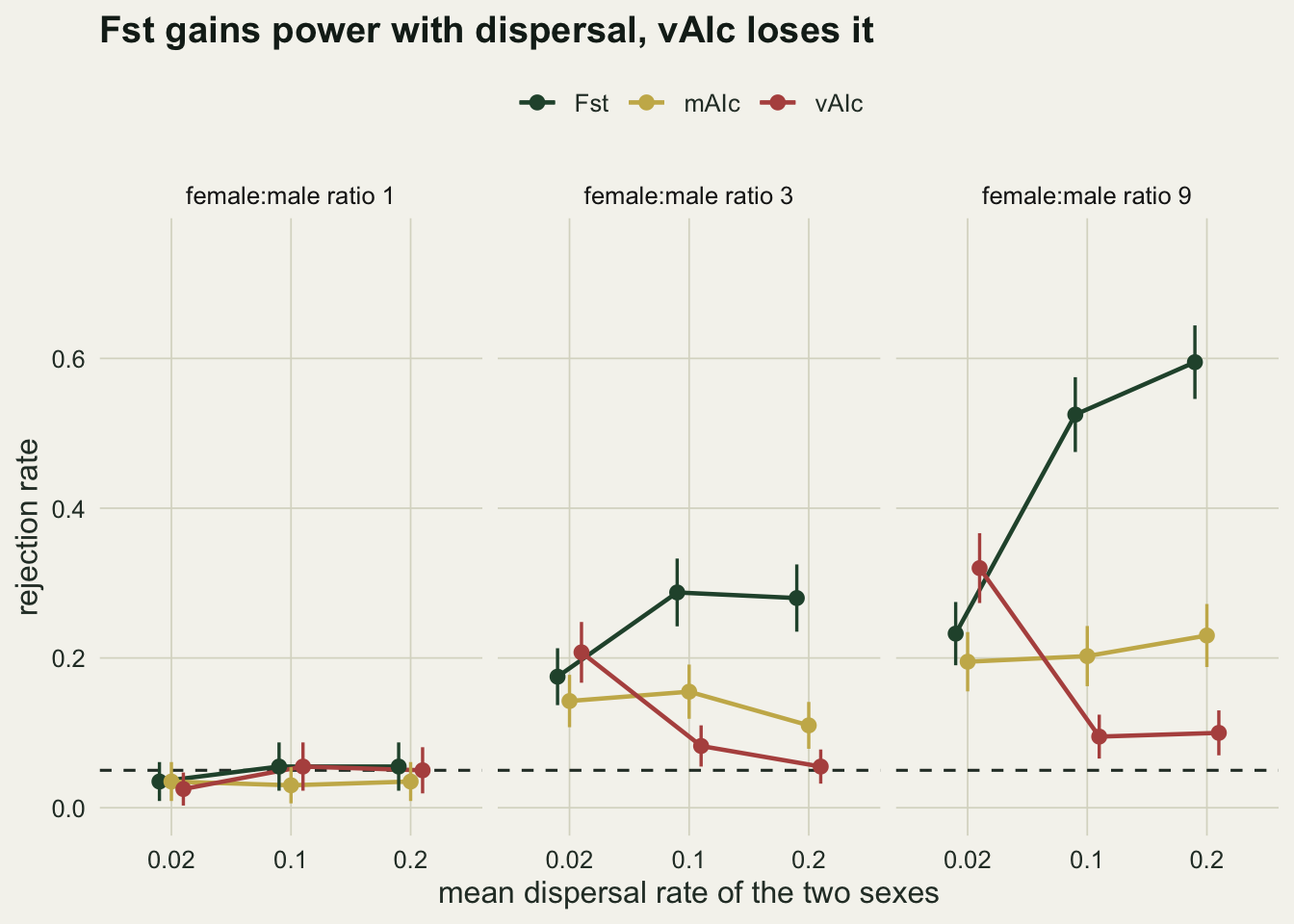
Why the number of immigrants is only a rough guide
A natural guess is that power depends on how many immigrants end up in the sample. The expected number among the 192 sampled animals of a sex is simply 192 times its dispersal rate, so the excess of female over male immigrants is arithmetic.
n_samp <- n_sex * n_deme
cells$imm_excess <- n_samp * (cells$d_f - cells$d_m)
biased <- cells[cells$ratio > 1, ]
ex_lo  <- biased[biased$ratio == 9 & biased$d_bar == 0.02, ]
ex_hi  <- biased[biased$ratio == 3 & biased$d_bar == 0.1, ]
ex_top <- biased[biased$ratio == 3 & biased$d_bar == 0.2, ]
ex_nine <- biased[biased$ratio == 9 & biased$d_bar == 0.1, ]
rank_cor <- cor(biased$imm_excess, biased$pow_fst, method = "spearman")
n_disc  <- sum(outer(biased$imm_excess, biased$imm_excess, "<") &
               outer(biased$pow_fst, biased$pow_fst, ">"))
n_pairs <- choose(nrow(biased), 2)
The expected excess ranks the six biased cells in roughly the order of their Fst power: the Spearman rank correlation is 0.83, and 2 of the 15 pairs of cells are out of order. One is the pair of three-fold cells at 0.1 and 0.2, which lie within Monte Carlo error of each other. The other is clear: at three-fold bias and 0.2 the excess is 38.4, larger than the 30.7 of a nine-fold bias at 0.1, yet power is 0.280 against 0.525. The count of immigrants overstates what high dispersal adds, because each immigrant there differs less from the residents.
The size of the signal explains the mismatch. Take two gene copies from two different animals of one sex in one deme. If both are residents their correlation relative to the whole population is the adult F; if one is an immigrant it came from another deme and the correlation is about -F/(D - 1); if both are immigrants they share a natal deme with probability 1/(D - 1) and otherwise correlate like a resident and an immigrant. Adding these up gives the expected Fst of a sex sampled after dispersal, F [(1 - d)^2 - 2d(1 - d)/(D - 1) + d^2/(D - 1) - d^2 (D - 2)/(D - 1)^2], with F the true Fst of the adult demes (close to the island formula). The prediction needs no simulation of the sample.
k_sex <- function(d, D = n_deme) {
  (1 - d)^2 - 2 * d * (1 - d) / (D - 1) + d^2 / (D - 1) - d^2 * (D - 2) / (D - 1)^2
}
cells$f_adult <- vapply(grid_res, function(x) attr(x, "f_adult"), 0)
cells$f_island <- 1 / (1 + 4 * n_adult * cells$d_bar)
cells$pred_f  <- cells$f_adult * k_sex(cells$d_f)
cells$pred_m  <- cells$f_adult * k_sex(cells$d_m)
cells$pred_gap <- cells$pred_m - cells$pred_f
biased <- cells[cells$ratio > 1, ]
pred_err <- max(abs(c(biased$pred_f - biased$fst_f, biased$pred_m - biased$fst_m)))
gap3 <- range(biased$gap[biased$ratio == 3]); gap9 <- range(biased$gap[biased$ratio == 9])
lim3 <- (3 - 1) / ((3 + 1) * n_adult); lim9 <- (9 - 1) / ((9 + 1) * n_adult)
sd_lo9 <- biased$null_sd[biased$ratio == 9 & biased$d_bar == 0.02]
sd_hi9 <- biased$null_sd[biased$ratio == 9 & biased$d_bar == 0.2]
sd_lo <- biased$null_sd[biased$ratio == 3 & biased$d_bar == 0.02]
sd_hi <- biased$null_sd[biased$ratio == 3 & biased$d_bar == 0.2]
f_lo9 <- biased[biased$ratio == 9 & biased$d_bar == 0.02, ]
d4n <- 4 * n_adult * 0.02
Across the six biased cells the predicted female and male Fst differ from the simulated means by at most 0.0011; the prediction is a first order approximation, but it is close enough to show where the signal comes from. The gap between the sexes is what the test has to detect, and it barely moves with the level of dispersal: from 0.0043 to 0.0046 at a three-fold bias across a ten-fold range of mean dispersal, and from 0.0064 to 0.0074 at nine-fold. Where immigration is rare, each immigrant is very different but there are few of them; where it is common, there are many but they are barely different. For small rates and 4Nd well above one the two effects cancel, and the expected gap approaches (ratio - 1)/((ratio + 1) N), a function of the bias ratio and deme size only: 0.0050 for a three-fold and 0.0080 for a nine-fold bias with one hundred adults per deme, a little above the simulated gaps, because at mean dispersal 0.02 4Nd is only 8, and at 0.2 the rates are no longer small.
What does change with dispersal is the noise. The standard deviation of the Fst difference under permutation falls from 0.0071 at mean dispersal 0.02 to 0.0036 at 0.2 at a three-fold bias, and from 0.0072 to 0.0036 at nine-fold, so it depends on the level of dispersal and hardly at all on the bias. The sampling variance of theta shrinks with theta itself. A signal of fixed size against falling noise is why the Fst test gains power as dispersal rises, and why the immigrant count, which grows with both the bias and the dispersal level, overstates the gain from dispersal. Neither the ratio nor the dispersal level decides power alone: a nine-fold bias at 0.02 reached 0.233, below the 0.280 of a three-fold bias at 0.2. The vAIc test works in the other direction because it looks for outliers: a single immigrant from a strongly differentiated deme has an extreme index, and that tail disappears when demes are nearly alike.
The account can be checked directly. If the observed difference is roughly normal with the permutation standard deviation, a one sided test at 0.05 has power near pnorm(gap/sd - 1.645).
biased$pow_norm <- pnorm(biased$gap / biased$null_sd - qnorm(1 - alpha_lev))
sn_tab <- data.frame(ratio = biased$ratio, d_bar = biased$d_bar,
                     signal_to_noise = sprintf("%.2f", biased$gap / biased$null_sd),
                     power_normal = sprintf("%.3f", biased$pow_norm),
                     power_simulated = sprintf("%.3f", biased$pow_fst))
print(sn_tab, row.names = FALSE)
ratio d_bar signal_to_noise power_normal power_simulated
3 0.02 0.61 0.151 0.175
9 0.02 0.89 0.227 0.233
3 0.10 1.09 0.289 0.287
9 0.10 1.75 0.543 0.525
3 0.20 1.21 0.331 0.280
9 0.20 2.00 0.637 0.595sn_err <- max(abs(biased$pow_norm - biased$pow_fst))
sn_rank <- cor(biased$pow_norm, biased$pow_fst, method = "spearman")The normal prediction differs from the simulated power by at most 0.051 across the six cells, and ranks them with a Spearman correlation of 0.94 against the 0.83 of the immigrant excess.
sig_df <- data.frame(d_bar = rep(biased$d_bar, 2),
                     ratio = factor(rep(paste0(biased$ratio, "-fold"), 2)),
                     value = c(biased$gap, biased$null_sd),
                     what = rep(c("signal", "noise"), each = nrow(biased)))
pal_ratio <- c(`3-fold` = te_gold, `9-fold` = te_rust)
p_sig <- ggplot(biased, aes(d_bar, gap, colour = factor(paste0(ratio, "-fold")))) +
  geom_line(linewidth = 0.8) + geom_point(size = 2.4) +
  geom_point(aes(y = pred_gap), shape = 4, size = 3.2, stroke = 1.1, colour = te_ink) +
  scale_x_log10(breaks = c(0.02, 0.1, 0.2)) +
  scale_colour_manual(values = pal_ratio, name = "female bias") +
  scale_y_continuous(limits = c(0, NA)) +
  labs(x = "mean dispersal (log scale)", y = "male Fst minus female Fst",
       title = "Signal: flat in dispersal") +
  theme_datasheet() + theme(legend.position = "top")
p_noise <- ggplot(biased, aes(d_bar, null_sd, colour = factor(paste0(ratio, "-fold")))) +
  geom_line(linewidth = 0.8) + geom_point(size = 2.4) +
  scale_x_log10(breaks = c(0.02, 0.1, 0.2)) +
  scale_colour_manual(values = pal_ratio, name = "female bias") +
  scale_y_continuous(limits = c(0, NA)) +
  labs(x = "mean dispersal (log scale)", y = "permutation SD of the difference",
       title = "Noise: falls with dispersal") +
  theme_datasheet() + theme(legend.position = "top")
(p_sig | p_noise) + plot_annotation(theme = theme_datasheet())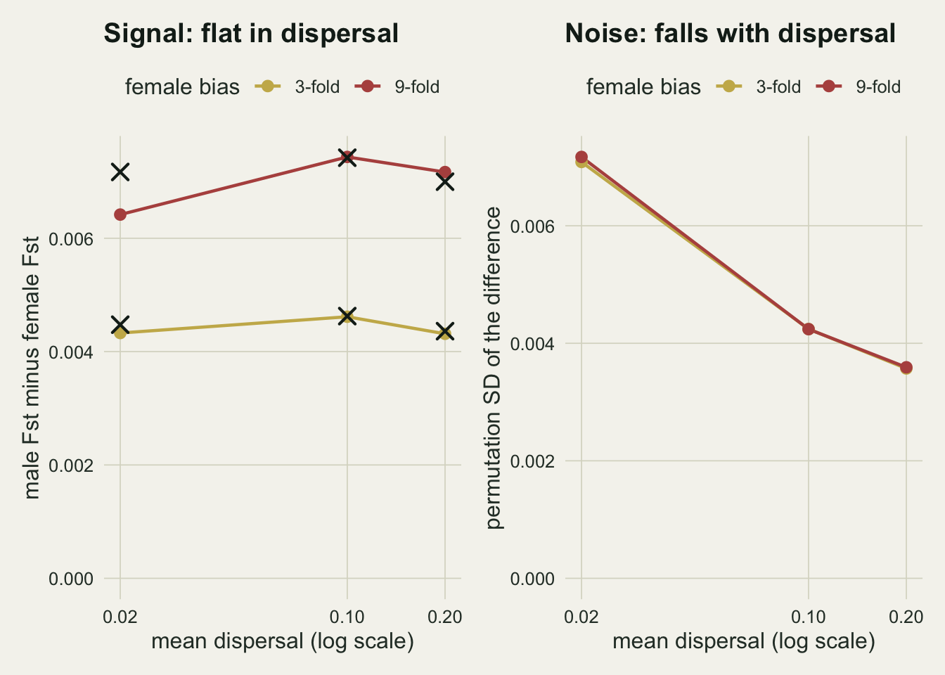
Loci, animals and the wrong life stage
The last measurements hold one cell fixed, female dispersal 0.15 and male 0.05, and change what the study collects: 30 or 200 SNPs instead of 60, 24 adults of each sex per deme instead of 12, and offspring genotyped before dispersal instead of dispersed adults. The offspring cell uses the nine-fold bias at the same mean rate (0.18 against 0.02), the strongest bias on the grid, so that any surviving signal would be easy to see. Each of these cells has 200 studies.
set.seed(4105)
eff_30   <- run_cell(200, 0.15, 0.05, n_loc = 30)
eff_200  <- run_cell(200, 0.15, 0.05, n_loc = 200)
eff_24   <- run_cell(200, 0.15, 0.05, n_per = 24)
eff_kids <- run_cell(200, 0.18, 0.02, stage = "offspring")
rate3 <- function(x) colMeans(x[, c("fst", "maic", "vaic")] <= alpha_lev)
r30 <- rate3(eff_30); r200 <- rate3(eff_200); r24 <- rate3(eff_24); rkid <- rate3(eff_kids)
base60 <- unlist(cells[cells$ratio == 3 & cells$d_bar == 0.1, c("pow_fst", "pow_maic", "pow_vaic")])
se_eff <- mcse(0.5, 200)
With the Fst test, 30 SNPs gave power 0.215, 60 gave 0.287 (from the grid) and 200 gave 0.470. Doubling the animals to 24 of each sex per deme, with 60 SNPs, gave 0.525, level with the 200 SNP panel within Monte Carlo error. The Monte Carlo standard error of these cells is at most 0.035. Sampling offspring instead of dispersed adults removed the signal: at the strongest bias on the grid the three tests rejected in 0.045, 0.060 and 0.070 of studies (Fst, mAIc, vAIc), at or below the nominal 0.05, where the same bias in dispersed adults gave Fst power of 0.525. Offspring are born where their parents bred, and nothing about an offspring’s genotype depends on its own sex, so the sex labels are exchangeable again.
eff_df <- data.frame(
  design = rep(c("30 SNPs, 12 per sex", "60 SNPs, 12 per sex", "200 SNPs, 12 per sex",
                 "60 SNPs, 24 per sex", "offspring, 60 SNPs, 12 per sex"), each = 3),
  stat = rep(c("Fst", "mAIc", "vAIc"), 5),
  power = c(r30, base60, r200, r24, rkid),
  n_rep = rep(c(200, 400, 200, 200, 200), each = 3))
eff_df$design <- factor(eff_df$design, levels = rev(unique(eff_df$design)))
eff_df$se <- mcse(eff_df$power, eff_df$n_rep)
ggplot(eff_df, aes(power, design, colour = stat)) +
  geom_vline(xintercept = alpha_lev, linetype = "dashed", colour = te_body) +
  geom_errorbar(aes(xmin = power - 2 * se, xmax = power + 2 * se), orientation = "y",
                width = 0, linewidth = 0.6, position = position_dodge(width = 0.6)) +
  geom_point(size = 2.4, position = position_dodge(width = 0.6)) +
  scale_colour_manual(values = c(Fst = te_forest, mAIc = te_gold, vAIc = te_rust), name = NULL) +
  labs(x = "rejection rate", y = NULL, title = "Twice the animals did as well as 200 SNPs") +
  theme_datasheet() + theme(legend.position = "top")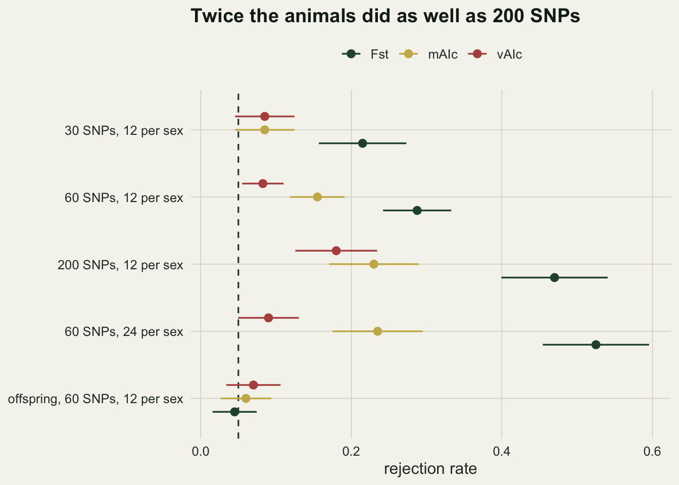
What to report
State when the animals were sampled relative to dispersal and breeding. The tests assume adults caught after dispersal and before they breed; offspring genotyped at the natal site carry no information on their own sex, and a sample that mixes stages dilutes the signal by the share of the wrong stage.
Say which direction was tested and why, and report all the statistics computed, not the one that came out significant. The three tests used here have very different power in different parts of the grid, so choosing the best one after seeing the p values inflates the error rate.
Report the realised Fst and the number of demes, animals per sex per deme and loci. The expected gap between the sexes is about (ratio - 1)/((ratio + 1) N), so with local deme sizes near one hundred the gap is a few thousandths in absolute Fst units, and the permutation noise at the study’s own Fst is the quantity that decides whether that gap could have been seen. Running the same tests on simulated data with the study’s design, as done above, gives the power directly, and a non-significant result should be read against that number rather than as evidence of equal dispersal.
Honest limits
The island model has sixteen equal demes of one hundred adults with random mating and no spatial structure. Real dispersal is mostly to neighbouring patches, so immigrants resemble the local deme more than an island immigrant does, and the signal is probably smaller than above; that case was not simulated. Deme size enters the expected gap directly through 1/N; the grid holds it fixed, and power at a deme size of twenty or of a thousand was not measured.
Dispersal is a single juvenile event with a fixed rate for each sex. Mortality of immigrants, dispersal by adults, and sampling that spans several cohorts all change the share of immigrants among the sampled animals; the offspring cell shows only the extreme case of sampling the wrong stage.
The markers are unlinked SNPs with starting frequencies between 0.1 and 0.9 and no genotyping error. Microsatellites with many alleles carry more information per locus, and the loci axis here cannot be translated into a number of microsatellites. Goudet, Perrin and Waser also considered statistics that are not implemented here, including Fis in each sex.
The corrected assignment index uses deme frequencies that include the animal being scored, which is the flattering choice described in the assignment post; it treats both sexes alike, so it weakens the contrast without biasing the test, and a leave-one-out version was not tried. The Fst of each sex is the Weir and Cockerham estimator applied to that sex’s twelve animals per deme; it is not the software implementation of any particular package, and its multilocus combination (ratio of summed components) is the one given by Weir and Cockerham.
The frequency-level burn-in was checked against the individual based model in one cell only, at mean dispersal 0.1; at 0.02 the burn-in is longest and its approach to equilibrium is least certain. The signal prediction uses the adult Fst that the burn-in actually produced, so it does not depend on that check.
Power in cells that differ by less than about two Monte Carlo standard errors should not be ranked. In particular, at three-fold bias the difference between mean dispersal 0.1 and 0.2 is within that band.
References
Goudet J, Perrin N, Waser P 2002 Molecular Ecology 11(6):1103-1114 (10.1046/j.1365-294X.2002.01496.x)
Prugnolle F, de Meeus T 2002 Heredity 88(3):161-165 (10.1038/sj.hdy.6800060)
Favre L, Balloux F, Goudet J, Perrin N 1997 Proceedings of the Royal Society B 264(1378):127-132 (10.1098/rspb.1997.0019)
Weir BS, Cockerham CC 1984 Evolution 38(6):1358-1370 (10.1111/j.1558-5646.1984.tb05657.x)