Downstream gene flow and the phantom dam

Headwater sites hold less genetic diversity than the mainstem with no barrier anywhere on the river. Simulating the false dam signal, and its repair, in R.

A dam sits on a lowland river. The genetic impact study samples thirty fish below it and thirty fish above it, scores twelve microsatellites in each, and compares expected heterozygosity locus by locus with a paired test. The site above the dam comes out lower, the test rejects, and the report says the dam has isolated the upstream population. Nothing in that design is exotic: one site below, one site above, a panel of markers and a paired test over loci.

The trouble is where the upstream site had to go. Suppose the reach sampled above the dam sits two network edges further up than the reach below it: fewer tributaries feeding it, smaller order, closer to a headwater. That is a design assumption in this post and not a survey of what published studies do, but it is the geometry a dam on a mainstem channel can force, because the impoundment itself is not a sampleable reach and the next tributary junction is above it. A headwater deme has one neighbour rather than three, and on a river the water carries eggs, larvae and drifting juveniles in one direction, so the deme sends more genes than it receives. Both of those lower its diversity, and both would do it on a river with no obstacle in it at all. The pattern has a name, the downstream increase in genetic diversity: Morrissey and de Kerckhove set out the theory for asymmetric gene flow in a dendritic network in 2009, Paz-Vinas and colleagues assembled the meta-analysis in 2015, and Thomaz, Christie and Knowles showed in 2016 how far network architecture alone moves the drift. This post is a demonstration of that known result, not a discovery of it. What it measures is the part a field worker has to price: how often the standard above-versus-below comparison flags a dam on a river that has none, at twelve and twenty-four loci and thirty fish a site, and what comparison does not.

The nearest thing on this site is checking a landscape genetics analysis. Its second check shows a barrier that cannot be separated from geographic distance, because the sites either side of a motorway sit in clusters that are also far apart, and it repairs that by sampling close to the barrier. Here the sites are already close: the two reaches either side of a dam can be a kilometre apart, and the confound is not distance but position in the network. No distance covariate removes it, because the two sites are at almost the same distance and at very different network positions. Its third check, on the lag between a landscape change and its genetic signal, is the other half of the argument and is used once below rather than repeated.

The other neighbours answer different questions. Drift, migration and isolation by distance runs a symmetric one-dimensional stepping stone and reads differentiation between demes, not diversity within them; its migration is the same in both directions and its line has no headwaters. Isolation by distance and by resistance compares distance metrics on a plane, where nothing is upstream of anything. The quantity here is within-deme heterozygosity, the geometry is a tree, and the migration matrix is not symmetric.

The post does four things. It writes the equilibrium heterozygosity of every deme as the solution of a linear system, so the gradient is arithmetic rather than a simulation result, and checks that a Wright-Fisher simulation lands on those values. It reads off how much of the gradient is set by the mutation rate and the exchange rate, which are the two numbers a paper rarely states. It puts a realistic genotyping effort on top of the simulation and measures how often the standard above-versus-below test rejects on an undammed river. Then it measures the comparison that should replace it.

library(ggplot2)
library(patchwork)

te_paper  <- "#f5f4ee"
te_ink    <- "#16241d"
te_body   <- "#2c3a31"
te_forest <- "#275139"
te_rust   <- "#b5534e"
te_gold   <- "#c9b458"
te_line   <- "#dad9ca"

theme_datasheet <- function() {
  theme_minimal(base_size = 12) +
    theme(plot.background  = element_rect(fill = te_paper, colour = NA),
          panel.background = element_rect(fill = te_paper, colour = NA),
          panel.grid.major = element_line(colour = te_line, linewidth = 0.3),
          panel.grid.minor = element_blank(),
          text             = element_text(colour = te_body),
          plot.title       = element_text(colour = te_ink, face = "bold"),
          plot.subtitle    = element_text(colour = te_body),
          axis.text        = element_text(colour = te_body))
}

The gradient is a linear solve

The river is a binary tree of fifteen demes. Deme one is the outlet, two demes sit at depth one, four at depth two and eight headwaters at depth three. Every edge is a reach of channel, and every deme holds the same number of diploids, so nothing in the design makes a headwater smaller or worse than the mainstem. The only asymmetries are the shape of the tree and the direction of the water.

Migration happens once a generation. A deme sends a fraction of its gene pool down its one downstream edge and receives along every edge that touches it. The per-edge downstream rate is m(1 + b)/2 and the upstream rate is m(1 - b)/2, so the total exchange rate on an edge is m whatever the bias b, and b moves only the direction. At b of zero the flow is symmetric and the only thing left is the shape of the tree; at b of nine tenths, nineteen migrants in twenty go downstream.

node_depth  <- c(0, 1, 1, 2, 2, 2, 2, 3, 3, 3, 3, 3, 3, 3, 3)
node_parent <- c(NA, 1, 1, 2, 2, 3, 3, 4, 4, 5, 5, 6, 6, 7, 7)
n_node      <- length(node_depth)
n_dip       <- 100
mut_rate    <- 2.5e-4
mig_rate    <- 0.1
bias_grid   <- c(0, 0.5, 0.9)
loci_grid   <- c(12, 24)
head_node   <- which(node_depth == 3)

mig_matrix <- function(m, b) {
  mm <- matrix(0, n_node, n_node)
  for (k in 2:n_node) {
    par_k <- node_parent[k]
    mm[par_k, k] <- m * (1 + b) / 2
    mm[k, par_k] <- m * (1 - b) / 2
  }
  diag(mm) <- 1 - rowSums(mm)
  mm
}

The life cycle is migration, then two-way mutation between the two alleles at rate u, then binomial sampling of 2N gene copies. Because that cycle is linear in the allele frequency except for the drift step, and the drift step has a known conditional variance, the second moments of the allele frequencies obey an exact linear recursion. Write Q for the matrix of expected products of allele frequencies, with entry i, j equal to the expectation of p_i times p_j. Migration maps Q to M Q M'. Mutation maps a frequency p to u + (1 - 2u) p, so it maps every entry of Q to u^2 + u(1 - 2u) plus (1 - 2u)^2 times the entry, using the fact that the mean frequency stays at one half at every deme and every generation. Drift leaves the off-diagonal entries alone, because the binomial draws in different demes are independent given the frequencies, and maps a diagonal entry to 0.5/(2N) + (1 - 1/(2N)) times itself. Setting the composition of the three equal to Q gives a linear system in the two hundred and twenty-five unknowns, and expected heterozygosity at a deme is one minus twice its diagonal entry.

he_exact <- function(m, b, u, n_ind = n_dip) {
  mm    <- mig_matrix(m, b)
  keep  <- 1 - 2 * u
  kron  <- kronecker(mm, mm)
  n_sq  <- n_node^2
  diag_ix <- (seq_len(n_node) - 1) * n_node + seq_len(n_node)
  drift_op <- diag(n_sq)
  diag(drift_op)[diag_ix] <- 1 - 1 / (2 * n_ind)
  mut_add  <- rep(u^2 + u * keep, n_sq)
  drift_add <- rep(0, n_sq)
  drift_add[diag_ix] <- 0.5 / (2 * n_ind)
  q_vec <- solve(diag(n_sq) - keep^2 * (drift_op %*% kron),
                 drift_op %*% mut_add + drift_add)
  1 - 2 * diag(matrix(q_vec, n_node, n_node))
}

exact_tab <- do.call(rbind, lapply(bias_grid, function(b) {
  he_b <- he_exact(mig_rate, b, mut_rate)
  data.frame(bias = b, node = seq_len(n_node), depth = node_depth, he = he_b)
}))
n_unknown <- n_node^2

ratio_exact <- vapply(bias_grid, function(b) {
  he_b <- he_exact(mig_rate, b, mut_rate)
  mean(he_b[head_node]) / he_b[1]
}, 0)
outlet_exact <- vapply(bias_grid, function(b) he_exact(mig_rate, b, mut_rate)[1], 0)
names(ratio_exact) <- names(outlet_exact) <- sprintf("b%.1f", bias_grid)

depth_he0  <- unname(tapply(exact_tab$he[exact_tab$bias == 0],
                            exact_tab$depth[exact_tab$bias == 0], mean))
step_out1  <- depth_he0[1] - depth_he0[2]
step_12    <- depth_he0[2] - depth_he0[3]
step_ratio <- step_12 / step_out1

With 100 diploids a deme, a per-edge exchange rate of 0.10 and a mutation rate of 0.00025, the solve over 225 unknowns gives a mean headwater heterozygosity of 0.935 times the outlet’s under symmetric gene flow. The difference is 6.5 per cent of the outlet’s diversity, with no barrier and no asymmetry anywhere in the model. It is not a degree effect, although the degrees do differ: a headwater sits on one edge, the outlet on two and the six internal demes on three. The solved values fall with depth instead, from 0.3692 at the outlet to 0.3688 at depth one, 0.3594 at depth two and 0.3452 at the headwaters. The outlet and the depth-one demes differ in degree and are 0.0004 apart; the depth-one and depth-two demes have the same three edges each and are 0.0094 apart, 22 times as far. Degree orders neither the values nor their spacing. What sets a deme’s equilibrium is how much of the rest of the network it exchanges with over many generations, and that falls from the root of the tree to its tips.

Adding a downstream bias of one half takes the ratio to 0.708, and a bias of nine tenths to 0.365. The bias does most of the work, which is the Morrissey and de Kerckhove point: the shape of the network alone produces a mild gradient, and it is asymmetric dispersal that turns it into something a study will see.

Nothing above is a simulation, and nothing above has a seed. Given the migration matrix, the deme size and the mutation rate, the gradient is fixed. The simulation that follows adds two things the solve cannot give: the spread of heterozygosity across loci within one river, which is what a paired test over twelve loci actually reads, and the extra noise of genotyping thirty fish.

q_step <- function(q_mat, mm, u, n_ind = n_dip) {
  keep  <- 1 - 2 * u
  q_mat <- mm %*% q_mat %*% t(mm)
  q_mat <- u^2 + u * keep + keep^2 * q_mat
  diag(q_mat) <- 0.5 / (2 * n_ind) + (1 - 1 / (2 * n_ind)) * diag(q_mat)
  q_mat
}
he_from_q <- function(q_mat) 1 - 2 * diag(q_mat)

mm_open <- mig_matrix(mig_rate, 0)
he_eq   <- he_exact(mig_rate, 0, mut_rate)

n_trace    <- 4000
within_pct <- 0.01
conv_tab <- do.call(rbind, lapply(bias_grid, function(b) {
  mm_b     <- mig_matrix(mig_rate, b)
  he_b     <- he_exact(mig_rate, b, mut_rate)
  ratio_b  <- mean(he_b[head_node]) / he_b[1]
  trace_ratio <- trace_outlet <- numeric(n_trace)
  q_trace <- matrix(0.25, n_node, n_node)
  for (g in seq_len(n_trace)) {
    q_trace <- q_step(q_trace, mm_b, mut_rate)
    he_g <- he_from_q(q_trace)
    trace_ratio[g]  <- mean(he_g[head_node]) / he_g[1]
    trace_outlet[g] <- he_g[1]
  }
  data.frame(bias = b,
             gen_ratio  = which(abs(trace_ratio / ratio_b - 1) < within_pct)[1],
             gen_outlet = which(abs(trace_outlet / he_b[1] - 1) < within_pct)[1])
}))
gen_ratio_worst  <- max(conv_tab$gen_ratio)
gen_outlet_worst <- max(conv_tab$gen_outlet)
bias_ratio_worst <- conv_tab$bias[which.max(conv_tab$gen_ratio)]
gen_ratio_open   <- conv_tab$gen_ratio[conv_tab$bias == 0]
gen_outlet_open  <- conv_tab$gen_outlet[conv_tab$bias == 0]

Starting every locus at a frequency of one half is a long way from equilibrium, so the run length has to be set before the simulation, from the same recursion, and checked at every bias the simulation uses rather than at one of them. Under symmetric flow the headwater to outlet ratio comes within one per cent of its solved value after 120 generations while the absolute heterozygosity at the outlet needs 2621: the shape of the gradient settles first and the level keeps falling. That order is not general. At a bias of 0.9 the ratio is the slower of the two, and over the three biases the worst cases are 1563 generations for the ratio and 2621 for the level. The run below uses a generation count above the slowest of all six.

run_river <- function(m, b, u, n_loci, n_gen, n_ind = n_dip) {
  mm <- mig_matrix(m, b)
  p  <- matrix(0.5, n_node, n_loci)
  for (g in seq_len(n_gen)) {
    p <- mm %*% p
    p <- u + (1 - 2 * u) * p
    p <- matrix(rbinom(n_node * n_loci, 2 * n_ind, p), n_node, n_loci) / (2 * n_ind)
  }
  p
}

n_gen  <- 3000
n_run  <- 5
n_loci <- 600
set.seed(2609)
freq_by_bias <- lapply(bias_grid, function(b) {
  do.call(cbind, lapply(seq_len(n_run), function(r)
    run_river(mig_rate, b, mut_rate, n_loci, n_gen)))
})
names(freq_by_bias) <- sprintf("b%.1f", bias_grid)
n_loci_tot <- n_run * n_loci
n_block12  <- n_loci_tot %/% loci_grid[1]
n_block24  <- n_loci_tot %/% loci_grid[2]

sim_tab <- do.call(rbind, lapply(seq_along(bias_grid), function(i) {
  he_i <- rowMeans(2 * freq_by_bias[[i]] * (1 - freq_by_bias[[i]]))
  data.frame(bias = bias_grid[i], node = seq_len(n_node),
             depth = node_depth, he = he_i)
}))
ratio_sim <- vapply(seq_along(bias_grid), function(i) {
  he_i <- sim_tab$he[sim_tab$bias == bias_grid[i]]
  mean(he_i[head_node]) / he_i[1]
}, 0)
outlet_sim <- vapply(seq_along(bias_grid), function(i)
  sim_tab$he[sim_tab$bias == bias_grid[i]][1], 0)
ratio_gap <- max(abs(ratio_sim - ratio_exact))
outlet_gap <- max(abs(outlet_sim / outlet_exact - 1))

The simulation ran 3000 independent biallelic loci for 3000 generations at each bias.

Simulated and solved values agree. The headwater to outlet ratios come out at 0.936, 0.711 and 0.365 against solved values of 0.935, 0.708 and 0.365, the largest gap being 0.0023. Outlet heterozygosity is within 0.4 per cent of the solved value at every bias. The linear system is the null, and the simulation is the sampling layer on top of it.

grad_exact <- aggregate(he ~ bias + depth, data = exact_tab, FUN = mean)
grad_sim   <- aggregate(he ~ bias + depth, data = sim_tab, FUN = mean)
grad_exact$lab <- factor(sprintf("%.1f", grad_exact$bias))
grad_sim$lab   <- factor(sprintf("%.1f", grad_sim$bias))

ggplot(grad_exact, aes(depth, he, colour = lab)) +
  geom_line(linewidth = 1) +
  geom_point(data = grad_sim, shape = 21, size = 3.2, stroke = 0.9,
             fill = te_paper) +
  scale_colour_manual(values = c(te_forest, te_gold, te_rust),
                      name = "downstream bias") +
  scale_x_continuous(breaks = 0:3,
                     labels = c("outlet", "depth 1", "depth 2", "headwater")) +
  labs(x = NULL, y = "expected heterozygosity",
       title = "The network makes the gradient on its own",
       subtitle = "lines: linear system; open points: simulation") +
  theme_datasheet() +
  theme(legend.position = "bottom")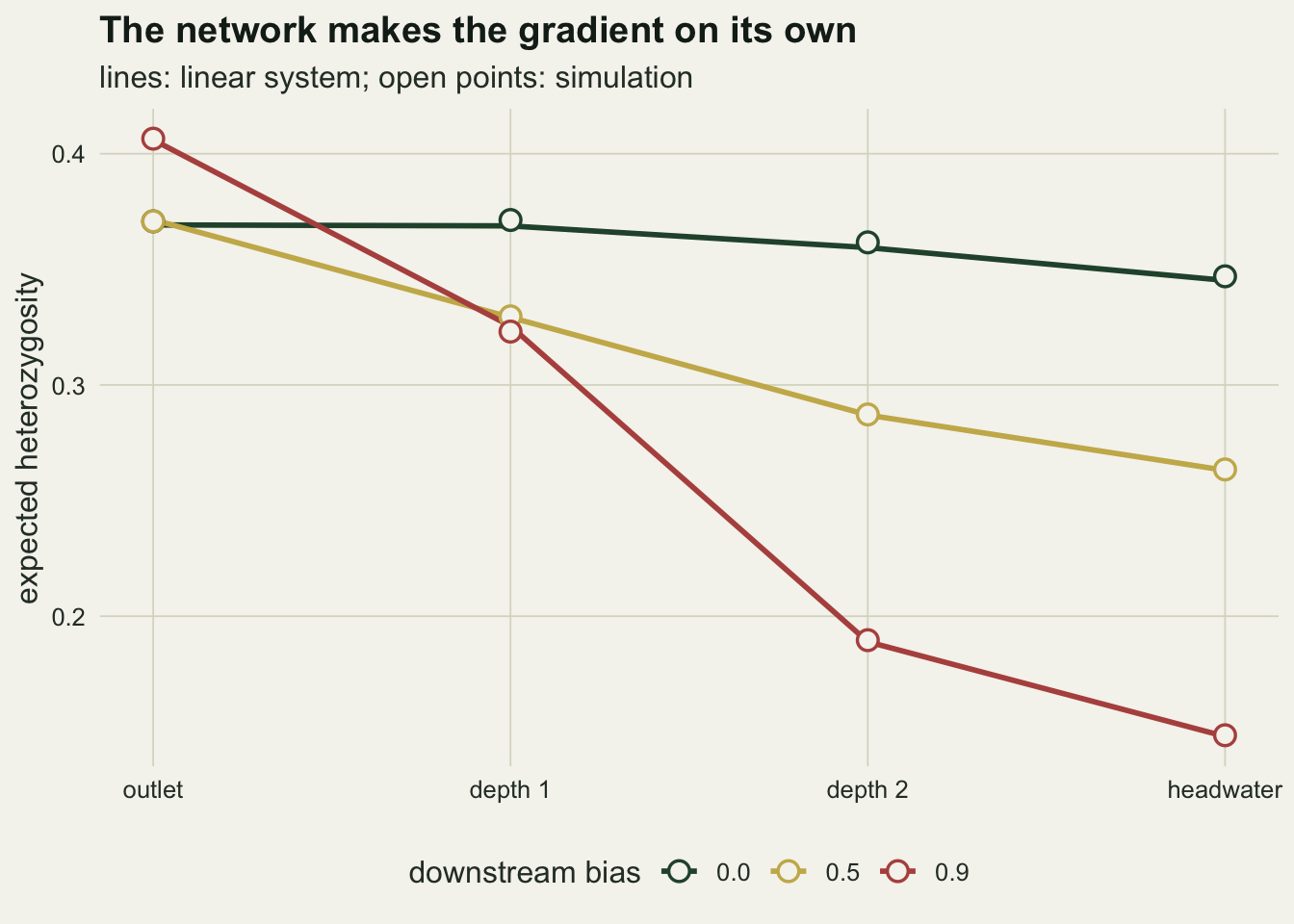

Figure 1: Expected heterozygosity by network depth under three downstream biases: lines from the linear system, points from the simulated rivers.

How much the ratio depends on mutation and migration

The headwater deficit is not a constant of rivers. It is a ratio of two equilibria, each set by the balance of drift against migration and mutation, so it moves with every one of those three. Since the solve is instant, the whole surface can be read off without simulating anything.

mut_grid <- c(1e-4, 2.5e-4, 5e-4, 1e-3, 2e-3, 5e-3)
mig_grid <- c(0.02, 0.05, 0.1, 0.2, 0.4)

sens_mut <- do.call(rbind, lapply(bias_grid, function(b)
  data.frame(bias = b, u = mut_grid,
             ratio = vapply(mut_grid, function(u) {
               he_b <- he_exact(mig_rate, b, u)
               mean(he_b[head_node]) / he_b[1] }, 0))))
sens_mig <- do.call(rbind, lapply(bias_grid, function(b)
  data.frame(bias = b, m = mig_grid,
             ratio = vapply(mig_grid, function(m) {
               he_b <- he_exact(m, b, mut_rate)
               mean(he_b[head_node]) / he_b[1] }, 0))))

pick <- function(tb, col, val, b) tb$ratio[tb[[col]] == val & tb$bias == b]
r_lo_mut <- pick(sens_mut, "u", min(mut_grid), 0.9)
r_hi_mut <- pick(sens_mut, "u", max(mut_grid), 0.9)
r_2e3    <- pick(sens_mut, "u", 2e-3, 0.9)
r_lo_mig <- pick(sens_mig, "m", min(mig_grid), 0)
r_hi_mig <- pick(sens_mig, "m", max(mig_grid), 0)
r_mig_b5_lo <- pick(sens_mig, "m", min(mig_grid), 0.5)
r_mig_b9_lo <- pick(sens_mig, "m", min(mig_grid), 0.9)

At a bias of nine tenths the headwater to outlet ratio runs from 0.223 at a mutation rate of 0.0001 to 0.860 at 0.005. That is the difference between a headwater with a fifth of the outlet’s diversity and one with six sevenths of it, from the mutation rate alone. Microsatellite rates sit at the top of that grid: at 0.002 the same river gives 0.742, against 0.365 at the 0.00025 used everywhere else in this post. Whether that moves the dam test as well, or only the number a paper reports, is measured in the next section. Any statement of the form “headwaters hold so many per cent of mainstem diversity” is a statement about the markers as much as about the river, and a ratio from one marker panel does not transfer to another.

The migration rate moves it the other way. Under symmetric flow the ratio runs from 0.803 at an exchange rate of 0.02 to 0.982 at 0.40: weak gene flow lets drift separate the demes and deepens the gradient, strong gene flow flattens it. Weak gene flow and a strong bias combine, and that combination is what a conservation genetics study is most likely to be looking at: a poorly connected catchment with a passive dispersal stage. At an exchange rate of 0.02 the headwaters carry 0.515 of the outlet’s heterozygosity at a bias of one half and 0.298 at nine tenths, with nothing blocking the channel.

sens_mut$lab <- factor(sprintf("%.1f", sens_mut$bias))
sens_mig$lab <- factor(sprintf("%.1f", sens_mig$bias))

p_mut <- ggplot(sens_mut, aes(u, ratio, colour = lab)) +
  geom_line(linewidth = 0.9) + geom_point(size = 2.2) +
  scale_x_log10() +
  scale_colour_manual(values = c(te_forest, te_gold, te_rust),
                      name = "downstream bias") +
  scale_y_continuous(limits = c(0.15, 1)) +
  labs(x = "mutation rate per allele per generation",
       y = "headwater / outlet heterozygosity",
       title = "Markers move the ratio") +
  theme_datasheet() +
  theme(legend.position = "bottom")

p_mig <- ggplot(sens_mig, aes(m, ratio, colour = lab)) +
  geom_line(linewidth = 0.9) + geom_point(size = 2.2) +
  scale_x_log10() +
  scale_colour_manual(values = c(te_forest, te_gold, te_rust),
                      name = "downstream bias") +
  scale_y_continuous(limits = c(0.15, 1)) +
  labs(x = "per-edge exchange rate", y = NULL,
       title = "So does connectivity") +
  theme_datasheet() +
  theme(legend.position = "bottom")

(p_mut | p_mig) + plot_layout(guides = "collect") +
  plot_annotation(theme = theme_datasheet()) &
  theme(legend.position = "bottom")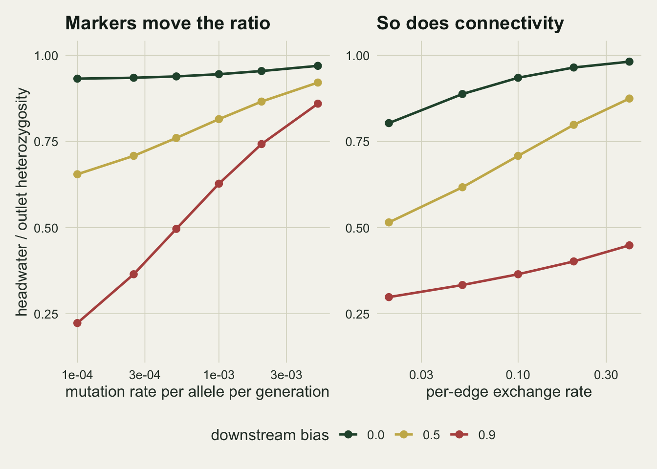

Figure 2: Headwater to outlet heterozygosity ratio from the linear system, against mutation rate and against the per-edge exchange rate.

A dam test on a river with no dam

Now the field layer. Thirty diploids are genotyped at a site, and expected heterozygosity is estimated per locus with the usual small-sample correction 2n/(2n - 1) of Nei 1978. The comparison is a one-sided paired t test over loci: the below-dam site is claimed to be the more diverse one, so the test asks whether the mean difference is positive. Three designs are run on exactly the same simulated rivers.

The naive design puts the below site on the mainstem at depth one and the above site at a headwater, two edges up, which is the assumption set out at the start. The mid-branch design moves the above site one edge back down, to depth two, which is what a worker who can reach a larger stream above the dam gets. The matched design abandons the mainstem site and compares the above-dam headwater with a headwater in a different branch of the same network, at the same depth.

Loci are independent given the demography, and the demography here is fixed, so each disjoint block of twelve or twenty-four loci from the simulated rivers is an independent replicate of the study. That is how the replication below is built: 3000 loci per bias become 250 independent twelve-locus studies or 125 twenty-four-locus studies.

n_fish  <- 30
site_below <- 2
site_head  <- 8
site_mid   <- 4
site_sister <- 12

sample_he <- function(p_vec, n_ind = n_fish) {
  x <- rbinom(length(p_vec), 2 * n_ind, p_vec) / (2 * n_ind)
  2 * x * (1 - x) * (2 * n_ind) / (2 * n_ind - 1)
}
flags_dam <- function(high_site, low_site) {
  t.test(high_site, low_site, paired = TRUE, alternative = "greater")$p.value < 0.05
}

set.seed(8814)
rate_tab <- do.call(rbind, lapply(seq_along(bias_grid), function(i) {
  p_mat <- freq_by_bias[[i]]
  do.call(rbind, lapply(loci_grid, function(nl) {
    blocks <- split(seq_len(ncol(p_mat)), rep(seq_len(ncol(p_mat) / nl), each = nl))
    hits <- vapply(blocks, function(ix) c(
      naive   = flags_dam(sample_he(p_mat[site_below, ix]),
                          sample_he(p_mat[site_head, ix])),
      mid     = flags_dam(sample_he(p_mat[site_below, ix]),
                          sample_he(p_mat[site_mid, ix])),
      matched = flags_dam(sample_he(p_mat[site_sister, ix]),
                          sample_he(p_mat[site_head, ix]))), numeric(3))
    data.frame(bias = bias_grid[i], loci = nl, n_study = length(blocks),
               design = rownames(hits), rate = rowMeans(hits))
  }))
}))
rate_tab$mc_se <- sqrt(rate_tab$rate * (1 - rate_tab$rate) / rate_tab$n_study)
rownames(rate_tab) <- NULL

get_rate <- function(d, b, nl) rate_tab$rate[rate_tab$design == d &
                                 rate_tab$bias == b & rate_tab$loci == nl]
se_max <- max(rate_tab$mc_se)
n_study12 <- rate_tab$n_study[rate_tab$loci == loci_grid[1]][1]
n_study24 <- rate_tab$n_study[rate_tab$loci == loci_grid[2]][1]
stopifnot(n_study12 == n_block12, n_study24 == n_block24)
matched_rng <- range(rate_tab$rate[rate_tab$design == "matched"])

he_b5      <- he_exact(mig_rate, 0.5, mut_rate)
def_naive5 <- 1 - he_b5[site_head] / he_b5[site_below]
def_mid5   <- 1 - he_b5[site_mid] / he_b5[site_below]

On a river with symmetric gene flow and no barrier, the naive design rejects in 0.164 of twelve-locus studies and 0.224 of twenty-four-locus studies. Those are not size violations. The matched design below holds its five per cent on the same simulated rivers, so the test is calibrated; the difference it finds between these two sites is real, because the shape gradient at 0.935 is real. What is false is the dam. More loci therefore find the gradient more often, and the second rate is larger than the first, a gap the power calculation later in this section turns from a Monte Carlo margin into an identity. Reading these rejections as a barrier is a genuine error and a contained one; it takes a downstream bias to make it large.

A downstream bias changes that. At a bias of one half the naive design flags a dam in 0.388 of twelve-locus studies and 0.688 of twenty-four-locus studies; at nine tenths it reaches 0.844 and 0.992. The Monte Carlo standard error is at most 0.045 on 250 twelve-locus and 125 twenty-four-locus studies per cell, which was fixed before the run. On a catchment where the dispersing stage drifts, a twenty-four-locus study of a river with nothing in it is more likely than not to report a barrier effect.

Moving the upstream site one edge closer helps but does not fix it. The mid-branch design rejects in 0.288 and 0.544 of studies at a bias of one half, against 0.388 and 0.688 for the naive one. The gradient is continuous in network position, and the solved deficit between the paired sites falls from 0.201 for the naive pair to 0.128 for the mid-branch pair. Moving the site down one edge removes part of the confound, and doubling the number of loci then puts the rejection rate back above where the worse siting started.

Why twelve loci are often not enough, and twenty-four often are, is visible in the per-locus differences themselves. Sample both sites at every simulated locus and look at the difference the paired test averages over.

set.seed(4407)
diff_tab <- do.call(rbind, lapply(seq_along(bias_grid), function(i) {
  p_mat <- freq_by_bias[[i]]
  data.frame(bias = bias_grid[i],
             gap = sample_he(p_mat[site_below, ]) - sample_he(p_mat[site_head, ]))
}))
eff_tab <- do.call(rbind, lapply(bias_grid, function(b) {
  d <- diff_tab$gap[diff_tab$bias == b]
  data.frame(bias = b, mean_gap = mean(d), sd_gap = sd(d),
             std_eff = mean(d) / sd(d), frac_neg = mean(d < 0))
}))

t_power <- function(ss, nl)
  pt(qt(0.95, nl - 1), nl - 1, ncp = sqrt(nl) * ss, lower.tail = FALSE)
pred_rate <- function(b, nl) t_power(eff_tab$std_eff[eff_tab$bias == b], nl)
pred_tab <- expand.grid(bias = bias_grid, loci = loci_grid)
pred_tab$predicted <- mapply(pred_rate, pred_tab$bias, pred_tab$loci)
pred_tab$measured  <- mapply(function(b, nl) get_rate("naive", b, nl),
                             pred_tab$bias, pred_tab$loci)
pred_gap <- max(abs(pred_tab$predicted - pred_tab$measured))
get_eff <- function(b, col) eff_tab[[col]][eff_tab$bias == b]

fixed_head <- vapply(seq_along(bias_grid), function(i)
  mean(sample_he(freq_by_bias[[i]][site_head, ]) == 0), 0)
fixed_below <- vapply(seq_along(bias_grid), function(i)
  mean(sample_he(freq_by_bias[[i]][site_below, ]) == 0), 0)

Under symmetric gene flow the mean difference between the mainstem site and the headwater is 0.0271, and the standard deviation of that difference across loci is 0.126: 39 per cent of loci point the wrong way. The standardised effect is 0.215, which is exactly the quantity a paired t test converts into power. At a bias of one half the mean difference rises to 0.0677 against a spread of 0.157, a standardised effect of 0.431, and at nine tenths it reaches 0.799.

Those three numbers account for every rejection rate the naive design produced. Feeding them into the noncentral t distribution, with no simulation of the test at all, predicts rejection rates that differ from the measured ones by at most 0.043. So the false flag is not a quirk of the test: it is an ordinary power calculation applied to a mean difference that should not have been there, and the only lever a study has over it is the number of loci, which makes the problem worse rather than better.

That power calculation also settles the marker question left open above. The ratio moved a long way with the mutation rate; what a design needs to know is whether the test moves with it. Rerunning the whole simulation at the microsatellite end of the grid answers that directly.

u_micro <- 2e-3
set.seed(7715)
micro_tab <- do.call(rbind, lapply(c(0.5, 0.9), function(b) {
  p_mat <- run_river(mig_rate, b, u_micro, n_loci_tot, n_gen)
  gap   <- sample_he(p_mat[site_below, ]) - sample_he(p_mat[site_head, ])
  ss    <- mean(gap) / sd(gap)
  he_b  <- he_exact(mig_rate, b, u_micro)
  data.frame(bias = b, ratio = mean(he_b[head_node]) / he_b[1], std_eff = ss,
             rate_lo = t_power(ss, loci_grid[1]),
             rate_hi = t_power(ss, loci_grid[2]))
}))
get_micro <- function(b, col) micro_tab[[col]][micro_tab$bias == b]

At a mutation rate of 0.002 and a bias of one half the standardised per-locus effect is 0.451, against 0.431 at the rate used everywhere else, and the predicted twelve-locus rejection rate is 0.428 against 0.404. The headwater to outlet ratio over that same change in the mutation rate runs from 0.708 to 0.866. At a bias of nine tenths the marker class does cost the test something: the effect falls from 0.799 to 0.627 and the predicted twelve-locus rate from 0.828 to 0.653, with twenty-four loci at 0.909. Raising the mutation rate lifts heterozygosity at both sites, so the ratio between them closes sharply, while the standardised difference the test reads comes out slightly larger at a bias of one half and about a fifth smaller at nine tenths. A panel with a higher mutation rate reports a milder headwater deficit and still flags the dam. The marker caveat belongs on the reported ratio, not on the false alarm.

The shape of the distribution at the strongest bias is worth a second look. It carries a second mode near one half, which is loci that are monomorphic in the headwater sample while the mainstem still carries both alleles: 45 per cent of headwater loci return a sampled heterozygosity of exactly zero at a bias of nine tenths, against 9 per cent at the mainstem site and 4 per cent at the headwater under symmetric flow. A field worker who sees a run of monomorphic loci above a dam is seeing something real; the question the design has to answer is whether the dam or the position put them there.

diff_tab$lab <- factor(sprintf("%.1f", diff_tab$bias))

ggplot(diff_tab, aes(gap, colour = lab)) +
  geom_vline(xintercept = 0, linetype = "dashed",
             colour = te_body, linewidth = 0.6) +
  geom_line(stat = "density", linewidth = 0.9) +
  scale_colour_manual(values = c(te_forest, te_gold, te_rust),
                      name = "downstream bias") +
  labs(x = "mainstem minus headwater, sampled heterozygosity at one locus",
       y = "density",
       title = "One locus decides almost nothing",
       subtitle = "thirty diploids a site; dashed line: no difference") +
  theme_datasheet() +
  theme(legend.position = "bottom")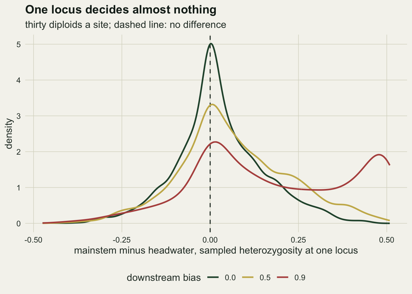

Figure 3: Distribution across loci of the sampled heterozygosity difference between the mainstem site and the headwater site, under three downstream biases.

The repair is a matched position, not a covariate

The matched design compares the site above the dam with a site of the same network position elsewhere in the catchment. It holds its level everywhere: the rejection rate stays between 0.032 and 0.088 across all three biases and both locus counts, against a nominal five per cent. That is the point of the whole exercise. The network gradient is a function of position, so a comparison between two demes at the same position has no gradient in it, and the test recovers the level it claims. Nothing about the strength of the downstream bias enters, because nothing has to be estimated or corrected: the confound is removed by where the second sample is taken.

A distance covariate cannot do the same job. The two sites either side of a dam are close together, and the headwater and the mainstem reach used in the naive design here are two edges apart, which is short. Distance is not the variable that differs between them; network position and flow direction are. That is the contrast with the second check in checking a landscape genetics analysis, where the barrier and the distance were nearly the same variable and the repair was to sample short cross-barrier pairs. Here short pairs are already available and do not help, because the confound survives at any distance.

rate_tab$design_lab <- factor(rate_tab$design,
  levels = c("naive", "mid", "matched"),
  labels = c("naive: mainstem vs headwater", "mid-branch: mainstem vs depth 2",
             "matched: headwater vs headwater"))
rate_tab$loci_lab <- factor(sprintf("%d loci", rate_tab$loci),
                            levels = sprintf("%d loci", loci_grid))

ggplot(rate_tab, aes(factor(bias), rate, fill = design_lab)) +
  geom_hline(yintercept = 0.05, linetype = "dashed",
             colour = te_body, linewidth = 0.6) +
  geom_col(position = position_dodge(width = 0.8), width = 0.72) +
  geom_errorbar(aes(ymin = rate - mc_se, ymax = rate + mc_se),
                position = position_dodge(width = 0.8), width = 0.2,
                colour = te_ink, linewidth = 0.4) +
  facet_wrap(~ loci_lab) +
  scale_fill_manual(values = c(te_forest, te_gold, te_rust), name = NULL) +
  scale_y_continuous(limits = c(0, 1)) +
  labs(x = "downstream bias", y = "rejection rate",
       title = "A dam flagged on a river with no dam",
       subtitle = "dashed line: the nominal five per cent level") +
  theme_datasheet() +
  theme(legend.position = "bottom",
        strip.text = element_text(colour = te_ink)) +
  guides(fill = guide_legend(nrow = 2))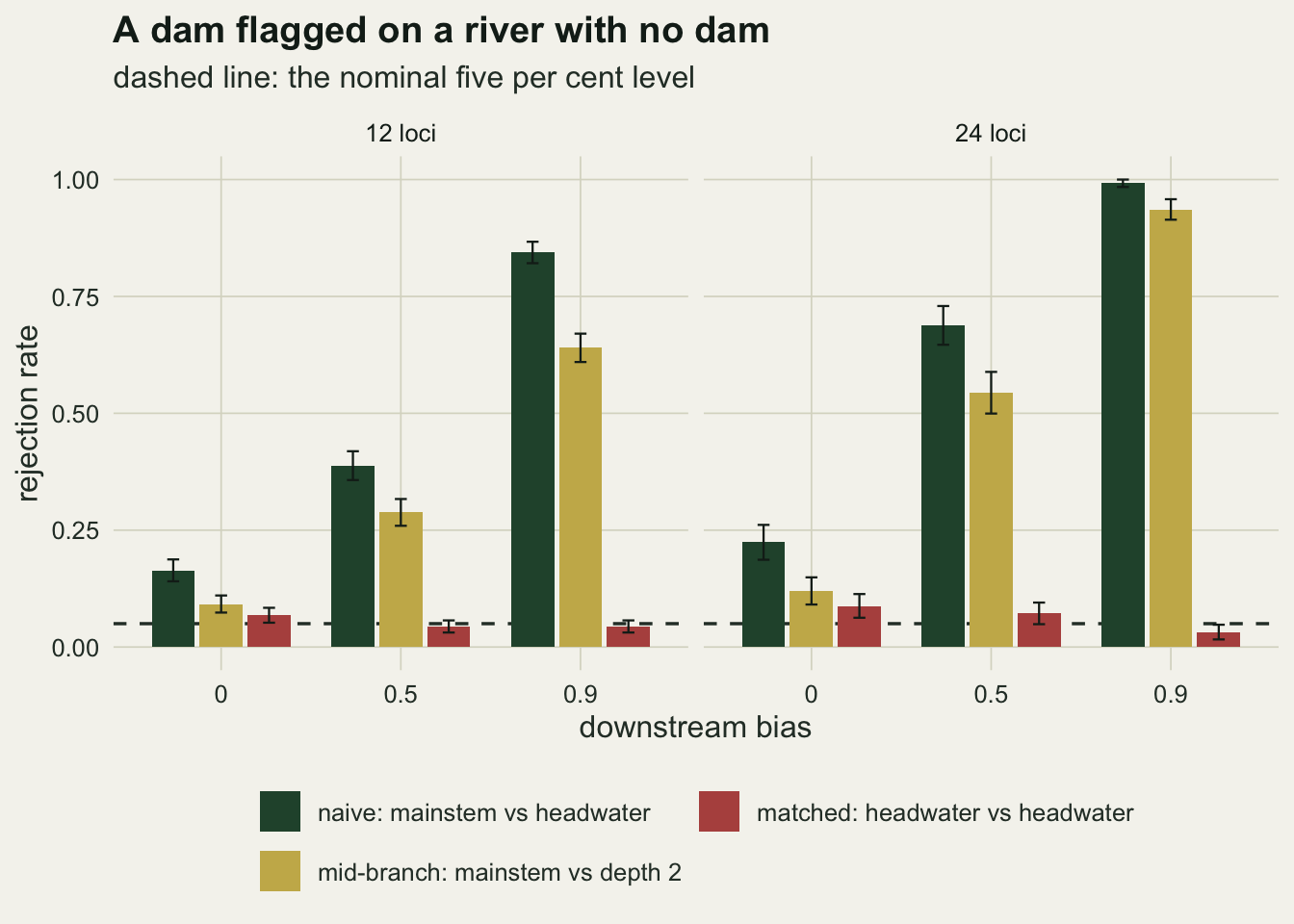

Figure 4: Rejection rate of a one-sided paired heterozygosity test on an undammed river, by downstream bias, comparison design and number of loci.

A real dam does eventually write something on top of all this, and the same linear recursion prices the wait. Iterate the map forward from the undammed equilibrium with one edge closed and watch the deficit between the two demes it separates.

q_now <- matrix(0.25, n_node, n_node)
for (g in seq_len(20000)) q_now <- q_step(q_now, mm_open, mut_rate)
he_open <- he_from_q(q_now)
def_nat <- 1 - he_open[site_mid] / he_open[site_below]

mm_dam <- mm_open
mm_dam[site_below, site_mid] <- 0
mm_dam[site_mid, site_below] <- 0
diag(mm_dam) <- 0
diag(mm_dam) <- 1 - rowSums(mm_dam)

n_lag   <- 300
def_path <- numeric(n_lag)
q_dam <- q_now
for (g in seq_len(n_lag)) {
  q_dam <- q_step(q_dam, mm_dam, mut_rate)
  he_g  <- he_from_q(q_dam)
  def_path[g] <- 1 - he_g[site_mid] / he_g[site_below]
}
gen_double <- which(def_path >= 2 * def_nat)[1]
gen_head   <- which(def_path >= 1 - ratio_exact[1])[1]
def_100    <- def_path[100]

Between the two demes the dam separates, the barrier-free deficit under symmetric flow is 0.0254. Closing the edge doubles it after 18 generations, and after 32 generations the deficit across one dammed edge exceeds the 0.0650 the network puts between its outlet and its headwaters unaided. By a hundred generations the deficit reaches 0.1267. For a fish with a three year generation time that is 96 years of concrete before the dam’s own mark outweighs the network’s, which is the same kind of lag the third check in checking a landscape genetics analysis measures for a lattice and a road, on a different statistic. The two errors point in opposite directions and both are live: a recent dam is too young to show, and an old river is already sloped.

What to report

Report the network position of every site, not just its coordinates. Stream order, distance from the outlet in edges, and the number of confluences above and below the reach are the variables the gradient runs on, and none of them is recoverable from a latitude and longitude pair. A table of sites with their positions lets a reader see the confound that a map of dots hides.

Pair sites by position when the question is a barrier. The matched comparison here held its nominal level at every bias, from 0.032 to 0.088, while the naive one reached 0.992. If the reach above a dam is a second-order headwater, the comparison it needs is with other second-order headwaters in the same catchment, and the below-dam mainstem site is the wrong reference whatever its distance.

State the marker class and the assumed mutation rate next to any diversity ratio. The same simulated river gives a headwater to outlet ratio of 0.223 at a mutation rate of 0.0001 and 0.860 at 0.005 under the same bias. Two marker panels with different mutation rates give different ratios from the same fish, and neither ratio transfers to a catchment with different connectivity. The dam test itself is far less sensitive to the marker class than the ratio is, so a faster-mutating panel reports a milder deficit without being any safer from the confound.

Give the age of the barrier in generations, not years. A dam takes 32 generations in this model to write a deficit across one edge as large as the one the undammed network already carries from outlet to headwater. A null result from a structure built two generations ago is a statement about power, not about passability.

Honest limits

The demes are equal in size. Real headwater reaches hold fewer fish than mainstem reaches, often far fewer, and a smaller deme drifts faster, so the true gradient on most rivers is steeper than this model’s. That makes the false alarm rates here conservative as estimates of the field problem and useless as estimates of the true ratio: the ratio reported above is the part attributable to shape and direction alone, with the size effect deliberately switched off so it cannot be mistaken for it.

The network is a regular binary tree with every headwater at the same depth. Real catchments are irregular, and the position-matched comparison is correspondingly harder to build: two second-order streams in one catchment can differ in the number of confluences between them and the sea, in their own upstream branching, and in local deme size. The matched design keeps its level here because the match is exact by construction. In the field it is approximate, and the residual mismatch is a residual gradient that nothing in the analysis reports.

Loci are biallelic and unlinked. That makes expected heterozygosity the only diversity measure available, and it rules out allelic richness, which the bottleneck literature and bottlenecks and genetic diversity both show responds faster to a loss of individuals than heterozygosity does. Whether allelic richness leads heterozygosity down the network gradient as well is a question a multi-allele model would have to answer, and a study that measures both may see them disagree.

The mutation model is symmetric and two-way between two alleles, which is a crude caricature of both marker classes a river study uses. Real single nucleotide polymorphism rates are orders of magnitude below the bottom of the mutation grid, and a panel of them is ascertained for being variable somewhere, which the model has no way to represent; a microsatellite mutates stepwise among many alleles, and a stepwise model reaches a different equilibrium heterozygosity at the same rate. The second figure should be read as a statement about how much the ratio moves when the mutation rate moves, not as a calibrated prediction for either marker.

Dispersal is a single number a generation and does not distinguish life stages. Real downstream bias is a property of a stage: drifting larvae and seeds go one way, adult fish swim both, and the effective bias depends on which stage disperses and how far. The biases used here span a wide range precisely because that number is rarely measured, and a study with direct movement data should use its own rather than any of these.

The test is the one the field uses, a one-sided paired t over loci, and its nominal level is not exact even under the matched design, because per-locus heterozygosity estimates are bounded, skewed and not normal. The matched rates measured above, 0.032 to 0.088 against a nominal five per cent, include whatever that approximation costs; the point of the comparison is the difference between designs, and both designs pay the same approximation.

Only one barrier scenario was run forward, a hard closure of a single edge under symmetric gene flow. A partially passable dam, a dam that also changes deme size by drowning a reach, and a dam on a river that already has a downstream bias would all give different lags, and the last of those is the common case.

References

Morrissey MB, de Kerckhove DT 2009 American Naturalist 174(6):875-889 (10.1086/648311)

Paz-Vinas I, Loot G, Stevens VM, Blanchet S 2015 Molecular Ecology 24(18):4586-4604 (10.1111/mec.13345)

Thomaz AT, Christie MR, Knowles LL 2016 Evolution 70(3):731-739 (10.1111/evo.12883)

Nei M 1978 Genetics 89(3):583-590 (10.1093/genetics/89.3.583)

Related tutorials

• Checking a landscape genetics analysis
• Drift, migration and isolation by distance
• Isolation by distance and by resistance
• Bottlenecks and genetic diversity