Checking a landscape genetics analysis

Four checks for a landscape genetics study in R: count the independent units, tell barrier from distance, time the lag after fragmentation, price the markers.

A landscape genetics analysis takes a matrix of genetic distances, a matrix of landscape distances, and returns a coefficient, a p-value and often a chosen resistance surface. The three tutorials before this one built those pieces: linearised Fst against Euclidean, least-cost and resistance distance, permutation inference for distance matrices, and a search over resistance values. This one asks what would have to be true for the output to mean anything.

Four checks, each with a measurement on simulated data where the answer is known: count the independent observations, ask whether a barrier can be told apart from distance under your design, time how long a barrier takes to reach Fst, and price the genetic data.

library(ggplot2)

te_pal <- list(forest = "#275139", green = "#2f8f63", sage = "#93a87f",
               clay = "#b5534e", gold = "#cda23f", line = "#dad9ca",
               ink = "#16241d", paper = "#f5f4ee")

theme_te <- function() {
  theme_minimal(base_size = 12) +
    theme(panel.grid.minor = element_blank(),
          panel.grid.major = element_line(colour = "#e7e6dc"),
          plot.background = element_rect(fill = "#f5f4ee", colour = NA),
          panel.background = element_rect(fill = "#f5f4ee", colour = NA),
          plot.title = element_text(face = "bold", colour = te_pal$ink),
          axis.title = element_text(colour = "#2c3a31"))
}

Check 1: how many independent observations do you have?

Sample 15 sites and you have 105 pairs. Feed those 105 rows to lm and it will happily report 103 degrees of freedom, but the data contain 15 independent units, not 105. Every site appears in 14 pairs, so anything peculiar about one site (a recent bottleneck, a small census size, a bad DNA extraction batch) is smeared across 14 rows at once.

The consequence is measurable. Build a null case: the predictor is the Euclidean distance matrix between fixed coordinates, and the genetic distance is driven by a site-level effect unrelated to space, plus a little pair-level noise. There is nothing to find. Then watch what the naive t-statistic does across repeated draws, and compare it with the distribution from permuting site order.

set.seed(4791)
n_site <- 15
site_x <- runif(n_site, 0, 100)
site_y <- runif(n_site, 0, 100)
pairs_1 <- t(combn(n_site, 2))
aa <- pairs_1[, 1]
bb <- pairs_1[, 2]
n_pair <- nrow(pairs_1)
euclid <- sqrt((site_x[aa] - site_x[bb])^2 + (site_y[aa] - site_y[bb])^2)
euclid_z <- (euclid - mean(euclid)) / sd(euclid)

draw_null <- function() {
  site_effect <- rnorm(n_site)
  (site_effect[aa] + site_effect[bb]) / 2 + rnorm(n_pair, 0, 0.3)
}

to_square <- function(v) {
  out <- matrix(0, n_site, n_site)
  out[cbind(aa, bb)] <- v
  out[cbind(bb, aa)] <- v
  out
}

n_rep <- 400
t_naive <- numeric(n_rep)
se_naive <- numeric(n_rep)
t_perm <- numeric(n_rep)
slope_perm <- numeric(n_rep)
for (r in seq_len(n_rep)) {
  gen_d <- draw_null()
  cf <- summary(lm(gen_d ~ euclid_z))$coefficients
  t_naive[r] <- cf[2, "t value"]
  se_naive[r] <- cf[2, "Std. Error"]
  ord <- sample(n_site)
  gen_p <- to_square(gen_d)[ord, ord][cbind(aa, bb)]
  cf_p <- summary(lm(gen_p ~ euclid_z))$coefficients
  t_perm[r] <- cf_p[2, "t value"]
  slope_perm[r] <- cf_p[2, "Estimate"]
}

se_ratio <- mean(se_naive) / sd(slope_perm)
cat("sites:", n_site, " pairs:", n_pair, " pairs containing any one site:",
    n_site - 1, " residual df reported by lm:", n_pair - 2,
    " null replicates:", n_rep, "\n")

sites: 15  pairs: 105  pairs containing any one site: 14  residual df reported by lm: 103  null replicates: 400 

cat("spread of the naive t under the null:", round(sd(t_naive), 3),
    " permutation spread:", round(sd(t_perm), 3),
    " assumed by the test: 1\n")

spread of the naive t under the null: 1.895  permutation spread: 1.929  assumed by the test: 1

cat("rejection rate of the nominal 5 percent test:",
    round(100 * mean(abs(t_naive) > qt(0.975, n_pair - 2)), 1), "percent\n")

rejection rate of the nominal 5 percent test: 32 percent

cat("naive standard error over permutation spread:", round(se_ratio, 3),
    " implied effective sample size:", round(n_pair * se_ratio^2, 1), "\n")

naive standard error over permutation spread: 0.524  implied effective sample size: 28.8 

The naive t-statistic has a spread of 1.895 where the test assumes 1, and the permutation distribution agrees with the truth at 1.929. A nominal 5 percent test rejects the null 32 percent of the time. That is not a small correction; it is the difference between a result and a coincidence.

The last line prices it. The standard error lm reports is 0.524 times the real spread of the slope, so the 105 pairs carry the information of 28.8 independent observations: close to twice the number of sites, and nowhere near the number of pairs. Adding sites buys power; recomputing more pairs from the same sites does not.

This is why Mantel and MMRR permute site labels rather than trusting parametric output, and it is the one check in this post that costs nothing to run.

grid_x <- seq(-6, 6, length.out = 400)
dens_df <- rbind(
  data.frame(x = grid_x, y = dt(grid_x, n_pair - 2),
             source = "assumed by lm (103 df)"),
  data.frame(x = density(t_naive, from = -6, to = 6, n = 400)$x,
             y = density(t_naive, from = -6, to = 6, n = 400)$y,
             source = "simulated null, 400 draws"),
  data.frame(x = density(t_perm, from = -6, to = 6, n = 400)$x,
             y = density(t_perm, from = -6, to = 6, n = 400)$y,
             source = "permuted site order"))

ggplot(dens_df, aes(x, y, colour = source, linetype = source)) +
  geom_line(linewidth = 0.9) +
  scale_colour_manual(values = c("grey35", te_pal$forest, te_pal$clay),
                      name = NULL) +
  scale_linetype_manual(values = c("dashed", "solid", "solid"), name = NULL) +
  labs(title = "The pairs are not independent rows",
       subtitle = "15 sites, 105 pairs, genetic distance unrelated to the predictor",
       x = "t-statistic for the slope", y = "density") +
  theme_te() +
  theme(legend.position = "bottom")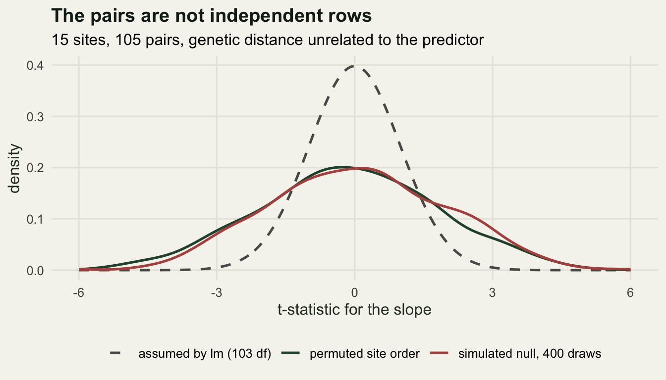

Figure 1: Null distribution of the t-statistic for a distance-matrix regression on 15 sites, compared with the reference distribution the naive test assumes.

Check 2: a barrier aligned with distance is not identifiable

A motorway, a river or a ridge usually separates sites that are also far apart, because the barrier is a line on the map and the sites sit in clusters either side of it. The barrier indicator and the geographic distance are then nearly the same variable, and no model selection can say which one drives the genetics.

The way to see this is to build two different truths on one set of coordinates and fit both models to each. Truth A: genetic distance is a function of Euclidean distance and nothing else. Truth B: genetic distance is a function of the barrier and nothing else. Both signals are standardised to the same strength, so the only thing that differs is which variable carries it.

build_sites <- function(add_near, seed) {
  set.seed(seed)
  xs <- c(runif(8, -11, -7), runif(8, 7, 11))
  ys <- runif(16, -6, 6)
  if (add_near) {
    xs <- c(xs, runif(4, -2.2, -0.6), runif(4, 0.6, 2.2))
    ys <- c(ys, runif(8, -6, 6))
  }
  n_s <- length(xs)
  pp <- t(combn(n_s, 2))
  sep <- sqrt((xs[pp[, 1]] - xs[pp[, 2]])^2 + (ys[pp[, 1]] - ys[pp[, 2]])^2)
  barrier <- as.numeric((xs[pp[, 1]] > 0) != (xs[pp[, 2]] > 0))
  list(n_s = n_s, n_pair = length(sep), sep = sep, barrier = barrier,
       sep_z = (sep - mean(sep)) / sd(sep),
       barrier_z = (barrier - mean(barrier)) / sd(barrier))
}

fit_both <- function(des, n_draw, effect, noise, seed) {
  set.seed(seed)
  out <- NULL
  for (truth in c("distance", "barrier")) {
    signal <- if (truth == "distance") des$sep_z else des$barrier_z
    r2_sep <- numeric(n_draw)
    r2_bar <- numeric(n_draw)
    for (r in seq_len(n_draw)) {
      gen_d <- effect * signal + rnorm(des$n_pair, 0, noise)
      r2_sep[r] <- summary(lm(gen_d ~ des$sep))$r.squared
      r2_bar[r] <- summary(lm(gen_d ~ des$barrier))$r.squared
    }
    out <- rbind(out, data.frame(
      truth = truth,
      distance_model = round(mean(r2_sep), 4),
      barrier_model = round(mean(r2_bar), 4),
      gap = round(mean(r2_sep) - mean(r2_bar), 4)))
  }
  out
}

designs <- list(`far clusters only` = build_sites(FALSE, 4801),
                `plus sites near the barrier` = build_sites(TRUE, 4801))
n_noise <- 200
conf_tab <- NULL
cat("noise draws per truth and design:", n_noise, "\n")

noise draws per truth and design: 200 

for (nm in names(designs)) {
  des <- designs[[nm]]
  cat(nm, ": sites", des$n_s, " pairs", des$n_pair,
      " correlation of distance with barrier",
      round(cor(des$sep, des$barrier), 4),
      " shortest cross-barrier pair", round(min(des$sep[des$barrier == 1]), 2),
      "\n")
  tb <- fit_both(des, n_noise, 0.8, 1, 4811)
  tb$design <- nm
  conf_tab <- rbind(conf_tab, tb)
}

far clusters only : sites 16  pairs 120  correlation of distance with barrier 0.9487  shortest cross-barrier pair 16.69 
plus sites near the barrier : sites 24  pairs 276  correlation of distance with barrier 0.6429  shortest cross-barrier pair 2.22 

print(conf_tab, row.names = FALSE)

    truth distance_model barrier_model     gap                      design
 distance         0.3915        0.3546  0.0369           far clusters only
  barrier         0.3461        0.3863 -0.0402           far clusters only
 distance         0.3924        0.1620  0.2304 plus sites near the barrier
  barrier         0.1650        0.3953 -0.2304 plus sites near the barrier

In the first design every cross-barrier pair is at least 16.69 units apart, all same-side pairs are closer, and the two predictors correlate at 0.9487. The r squared values then barely move when the truth changes: 0.3915 and 0.3546 when distance is the truth, 0.3461 and 0.3863 when the barrier is. The gap between the two models is 0.0369 one way and -0.0402 the other. A study of this shape can report that a barrier restricts gene flow while the same data are equally consistent with pure isolation by distance.

Now add eight more sites close to the barrier, half on each side. The correlation between the predictors falls to 0.6429, the shortest cross-barrier pair is 2.22 units, and the gap in r squared becomes 0.2304 in both directions, against 0.0369 and -0.0402 before. The two truths are now distinguishable.

Nothing statistical changed: same models, same noise. What changed is that the design now contains pairs of sites that are close together but on opposite sides, and those pairs are the only ones that carry information about the barrier as such. If your field season cannot produce them, no amount of AIC, commonality analysis or resistance optimisation will recover the distinction.

conf_long <- rbind(
  data.frame(truth = conf_tab$truth, design = conf_tab$design,
             r2 = conf_tab$distance_model, fitted = "distance model"),
  data.frame(truth = conf_tab$truth, design = conf_tab$design,
             r2 = conf_tab$barrier_model, fitted = "barrier model"))
conf_long$truth <- factor(conf_long$truth, levels = c("distance", "barrier"),
                          labels = c("distance is the truth",
                                     "barrier is the truth"))
conf_long$design <- factor(conf_long$design, levels = names(designs))

ggplot(conf_long, aes(truth, r2, fill = fitted)) +
  geom_col(position = position_dodge(width = 0.72), width = 0.6,
           colour = "white") +
  facet_wrap(~design) +
  scale_fill_manual(values = c(`distance model` = te_pal$forest,
                               `barrier model` = te_pal$clay), name = NULL) +
  labs(title = "Design decides whether the barrier is identifiable",
       subtitle = "mean r squared over 200 noise draws, equal signal strength",
       x = NULL, y = "r squared") +
  theme_te() +
  theme(legend.position = "bottom")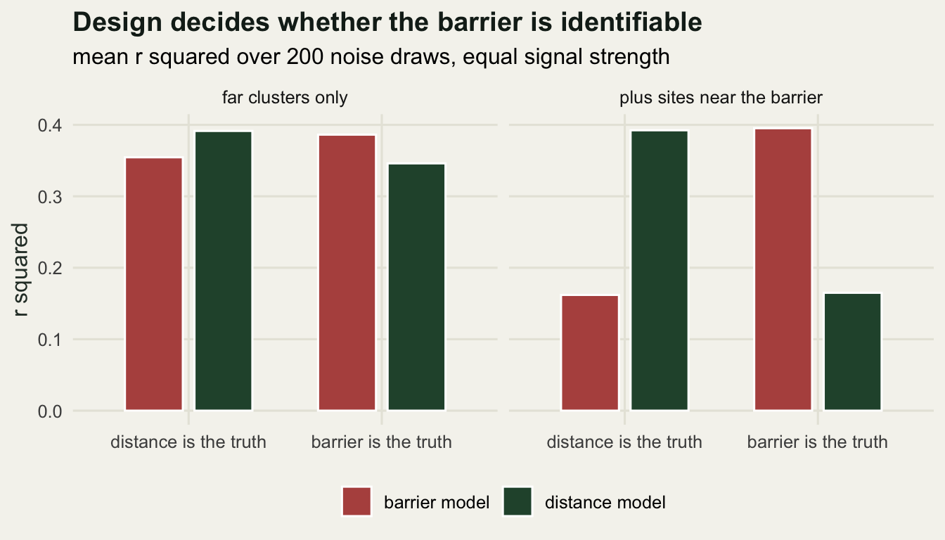

Figure 2: Mean r squared of the distance model and the barrier model under each of two truths, for a confounded design and for one with sites near the barrier.

Check 3: the time lag

Every Fst-based landscape genetics analysis assumes that drift and migration have settled into balance under the landscape you measured. Fragmentation is recent almost everywhere, so the assumption is usually false, and the question is how false.

Simulate it. A 16 by 16 lattice of demes, 50 diploids each, 60 biallelic loci, migration to rook neighbours only, binomial drift, and a small mutation rate so variation is not lost. Run it as a continuous landscape until the pattern is stationary, then drop a hard barrier between columns 8 and 9 and keep going. Forty-eight sites are sampled either side of the barrier, so short cross-barrier pairs are plentiful: check 2 says that is the only design in which the question can be asked.

n_side <- 16
n_deme <- n_side * n_side
n_dip <- 50
n_locus <- 200
mig_rate <- 0.05
mut_rate <- 1e-4
bar_col <- 8
deme_id <- matrix(seq_len(n_deme), n_side, n_side, byrow = TRUE)

build_mig <- function(blocked) {
  mm <- matrix(0, n_deme, n_deme)
  for (rr in seq_len(n_side)) {
    for (cc in seq_len(n_side)) {
      here <- deme_id[rr, cc]
      stay <- 1 - mig_rate
      nb <- list(c(rr - 1, cc), c(rr + 1, cc), c(rr, cc - 1), c(rr, cc + 1))
      for (v in nb) {
        ok <- v[1] >= 1 && v[1] <= n_side && v[2] >= 1 && v[2] <= n_side
        if (ok && blocked && ((cc <= bar_col) != (v[2] <= bar_col))) ok <- FALSE
        if (ok) {
          there <- deme_id[v[1], v[2]]
          mm[here, there] <- mm[here, there] + mig_rate / 4
        } else {
          stay <- stay + mig_rate / 4
        }
      }
      mm[here, here] <- stay
    }
  }
  mm
}

mig_open <- t(build_mig(FALSE))
mig_shut <- t(build_mig(TRUE))

step_gen <- function(freq, mig_t) {
  freq <- freq %*% mig_t
  freq <- freq * (1 - mut_rate) + (1 - freq) * mut_rate
  matrix(rbinom(length(freq), 2 * n_dip, as.vector(freq)),
         nrow = nrow(freq)) / (2 * n_dip)
}

site_row <- rep(seq(2, 16, 2), each = 6)
site_col <- rep(6:11, times = 8)
site_id <- deme_id[cbind(site_row, site_col)]
pairs_3 <- t(combn(length(site_id), 2))
uu <- pairs_3[, 1]
vv <- pairs_3[, 2]
geo <- sqrt((site_row[uu] - site_row[vv])^2 + (site_col[uu] - site_col[vv])^2)
crossed <- as.numeric((site_col[uu] <= bar_col) != (site_col[vv] <= bar_col))
geo_class <- round(geo, 3)
both_kinds <- tapply(crossed[geo <= 5], geo_class[geo <= 5],
                     function(z) length(unique(z)))
keep <- geo <= 5 & geo_class %in% as.numeric(names(which(both_kinds == 2)))

raw_fst <- function(freq) {
  fa <- freq[, uu, drop = FALSE]
  fb <- freq[, vv, drop = FALSE]
  h_s <- (2 * fa * (1 - fa) + 2 * fb * (1 - fb)) / 2
  f_bar <- (fa + fb) / 2
  h_t <- 2 * f_bar * (1 - f_bar)
  colSums(h_t - h_s) / colSums(h_t)
}

barrier_signal <- function(fst) {
  lin <- (fst / (1 - fst))[keep]
  cls <- geo_class[keep]
  cross_k <- crossed[keep]
  by_class <- tapply(seq_along(lin), cls, function(idx)
    mean(lin[idx][cross_k[idx] == 1]) - mean(lin[idx][cross_k[idx] == 0]))
  wts <- tapply(seq_along(lin), cls, length)
  m_geo <- lm(lin ~ cls)
  m_both <- lm(lin ~ cls + cross_k)
  c(diff = sum(by_class * wts) / sum(wts),
    gain = summary(m_both)$r.squared - summary(m_geo)$r.squared,
    tval = summary(m_both)$coefficients["cross_k", "t value"])
}

cat("lattice:", n_side, "by", n_side, " demes:", n_deme,
    " diploids per deme:", n_dip, " loci simulated:", n_locus,
    " loci used for this check: 60\n")

lattice: 16 by 16  demes: 256  diploids per deme: 50  loci simulated: 200  loci used for this check: 60

cat("barrier between columns", bar_col, "and", bar_col + 1, "\n")

barrier between columns 8 and 9 

cat("migration rate:", mig_rate, " mutation rate:", mut_rate,
    " drift clock 2N:", 2 * n_dip,
    " migration clock 1/(2m):", 1 / (2 * mig_rate), "\n")

migration rate: 0.05  mutation rate: 1e-04  drift clock 2N: 100  migration clock 1/(2m): 10 

cat("sampled sites:", length(site_id), " pairs used:", sum(keep),
    " of which cross-barrier:", sum(crossed[keep]),
    " matched distance classes:", length(unique(geo_class[keep])), "\n")

sampled sites: 48  pairs used: 428  of which cross-barrier: 146  matched distance classes: 7 

The barrier signal is the excess in linearised Fst of cross-barrier pairs over same-side pairs at the same geographic distance, averaged over the distance classes holding both kinds of pair. Matching on distance matters: without it the statistic just re-measures isolation by distance. Reported next to it is the r squared gained by adding the barrier term to a regression on distance alone.

set.seed(4821)
freq <- matrix(0.5, n_locus, n_deme)
for (g in seq_len(400)) freq <- step_gen(freq, mig_open)
freq_400 <- freq
for (g in seq_len(100)) freq <- step_gen(freq, mig_open)

for (nm in c("400", "500")) {
  ff <- if (nm == "400") freq_400 else freq
  sg <- barrier_signal(raw_fst(ff[1:60, site_id]))
  cat("continuous landscape, generation", nm,
      ": barrier excess", sprintf("%.4f", sg[["diff"]]),
      " r squared gain", sprintf("%.4f", sg[["gain"]]),
      " t value", sprintf("%.2f", sg[["tval"]]), "\n")
}

continuous landscape, generation 400 : barrier excess -0.0003  r squared gain 0.0000  t value -0.11 
continuous landscape, generation 500 : barrier excess -0.0002  r squared gain 0.0000  t value -0.00 

check_gen <- c(0, 5, 10, 25, 50, 100)
freq_now <- freq
gen_now <- 0
lag_tab <- NULL
for (target in check_gen) {
  while (gen_now < target) {
    freq_now <- step_gen(freq_now, mig_shut)
    gen_now <- gen_now + 1
  }
  sg <- barrier_signal(raw_fst(freq_now[1:60, site_id]))
  lag_tab <- rbind(lag_tab, data.frame(generation = target,
                                       barrier_excess = round(sg[["diff"]], 4),
                                       r2_gain = round(sg[["gain"]], 4),
                                       t_value = round(sg[["tval"]], 2)))
}
freq_frag <- freq_now
print(lag_tab, row.names = FALSE)

 generation barrier_excess r2_gain t_value
          0        -0.0002  0.0000    0.00
          5         0.0013  0.0009    0.75
         10         0.0018  0.0006    0.62
         25         0.0082  0.0162    3.12
         50         0.0172  0.0460    5.23
        100         0.0288  0.1366    9.23

Before the barrier exists the statistic is empty, as it should be: the excess is -0.0003 at generation 400 and -0.0002 at generation 500, with r squared gains of 0.0000 at both. That is the control, and it also shows the pattern is stationary over the last hundred generations of the run.

After fragmentation the signal arrives slowly. At 5 and 10 generations the excess is 0.0013 and 0.0018 with t values of 0.75 and 0.62: nothing a study would detect. It first becomes clear at 25 generations (excess 0.0082, t value 3.12), and it keeps growing to 0.0288 at 100 generations, where the barrier term adds 0.1366 to the r squared. The clock here is set by drift within a deme, 2N = 100 generations, and a quarter of that clock is what the barrier needed to become visible.

For a species with a generation time of five years, those 25 generations are more than a century of road. The honest reading of a null result from a road built in the 1990s is that the analysis had no power, not that the road is permeable.

freq_back <- freq_frag
gen_now <- 0
back_tab <- NULL
for (target in check_gen) {
  while (gen_now < target) {
    freq_back <- step_gen(freq_back, mig_open)
    gen_now <- gen_now + 1
  }
  sg <- barrier_signal(raw_fst(freq_back[1:60, site_id]))
  back_tab <- rbind(back_tab, data.frame(generation = target,
                                         barrier_excess = round(sg[["diff"]], 4),
                                         r2_gain = round(sg[["gain"]], 4),
                                         t_value = round(sg[["tval"]], 2)))
}
print(back_tab, row.names = FALSE)

 generation barrier_excess r2_gain t_value
          0         0.0288  0.1366    9.23
          5         0.0224  0.1120    8.69
         10         0.0196  0.0889    7.76
         25         0.0105  0.0353    5.07
         50         0.0023  0.0015    1.05
        100         0.0071  0.0246    4.24

The reverse case is the same argument with the sign flipped, and it need not be symmetric. Reopening the barrier erases the excess from 0.0288 to 0.0105 within 25 generations and to 0.0023 by 50, faster than it built up, because homogenisation runs on the migration clock of 1/(2m) = 10 generations while divergence ran on the drift clock of 100. Where gene flow is weaker the two clocks converge and an old barrier stays legible long after it is gone. Either way, Fst reports the landscape as it stood some decades back, not the one you mapped.

lag_long <- rbind(
  data.frame(generation = lag_tab$generation, value = lag_tab$barrier_excess,
             phase = "barrier inserted", stat = "excess in Fst / (1 - Fst)"),
  data.frame(generation = lag_tab$generation, value = lag_tab$r2_gain,
             phase = "barrier inserted", stat = "r squared gained"),
  data.frame(generation = back_tab$generation, value = back_tab$barrier_excess,
             phase = "barrier removed again", stat = "excess in Fst / (1 - Fst)"),
  data.frame(generation = back_tab$generation, value = back_tab$r2_gain,
             phase = "barrier removed again", stat = "r squared gained"))

ggplot(lag_long, aes(generation, value, colour = phase)) +
  geom_hline(yintercept = 0, colour = te_pal$line) +
  geom_line(linewidth = 0.9) +
  geom_point(size = 2.2) +
  facet_wrap(~stat, scales = "free_y") +
  scale_colour_manual(values = c(`barrier inserted` = te_pal$forest,
                                 `barrier removed again` = te_pal$clay),
                      name = NULL) +
  labs(title = "Fst lags the landscape it is asked about",
       subtitle = "16 by 16 lattice, N = 50, 60 loci, 48 sampled sites",
       x = "generations since the landscape changed", y = NULL) +
  theme_te() +
  theme(legend.position = "bottom")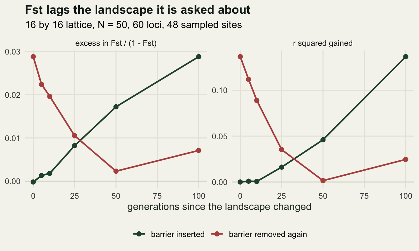

Figure 3: Cross-barrier excess in linearised Fst and the r squared gained by the barrier term, against generations since the landscape changed.

Check 4: how much genetic data does the precision need?

The response variable is itself an estimate. A pairwise Fst from 10 loci and 10 individuals per site is a noisy guess at a quantity 200 loci would pin down. So vary the amount of genetic data while holding the biology fixed, which the simulation allows because the true allele frequencies are known.

Take the fragmented populations at generation 100, sample individuals from them, and recompute everything for four locus counts and three sample sizes.

freq_site <- freq_frag[, site_id, drop = FALSE]
fit_stats <- function(fst) {
  lin <- (fst / (1 - fst))[keep]
  cls <- geo_class[keep]
  cross_k <- crossed[keep]
  fit <- lm(lin ~ cls + cross_k)
  c(slope = coef(fit)[[2]], barrier = coef(fit)[[3]],
    r2 = summary(fit)$r.squared)
}

true_fst <- raw_fst(freq_site)
true_stats <- fit_stats(true_fst)
cat("true frequencies, all 200 loci: mean pairwise Fst",
    round(mean(true_fst[keep]), 4), " distance slope",
    round(true_stats[["slope"]], 5), " barrier effect",
    round(true_stats[["barrier"]], 4), " r squared",
    round(true_stats[["r2"]], 4), "\n")

true frequencies, all 200 loci: mean pairwise Fst 0.0952  distance slope 0.00942  barrier effect 0.0226  r squared 0.4279 

set.seed(4831)
locus_set <- c(10, 30, 60, 200)
ind_set <- c(10, 30, 50)
n_draw <- 20
cat("locus counts:", locus_set, " individuals per site:", ind_set,
    " resampling draws per cell:", n_draw, "\n")

locus counts: 10 30 60 200  individuals per site: 10 30 50  resampling draws per cell: 20 

prec_tab <- NULL
for (n_ind in ind_set) {
  for (n_loc in locus_set) {
    fst_draws <- matrix(NA_real_, length(geo), n_draw)
    stat_draws <- matrix(NA_real_, n_draw, 3)
    for (r in seq_len(n_draw)) {
      sel <- if (n_loc == n_locus) seq_len(n_locus) else sample(n_locus, n_loc)
      sub_freq <- freq_site[sel, , drop = FALSE]
      obs <- matrix(rbinom(length(sub_freq), 2 * n_ind, as.vector(sub_freq)),
                    nrow = n_loc) / (2 * n_ind)
      fst_draws[, r] <- raw_fst(obs)
      stat_draws[r, ] <- fit_stats(fst_draws[, r])
    }
    prec_tab <- rbind(prec_tab, data.frame(
      loci = n_loc, individuals = n_ind,
      sd_one_fst = round(mean(apply(fst_draws[keep, ], 1, sd)), 4),
      distance_slope = round(mean(stat_draws[, 1]), 5),
      barrier_effect = round(mean(stat_draws[, 2]), 4),
      r_squared = round(mean(stat_draws[, 3]), 4)))
  }
}
print(prec_tab, row.names = FALSE)

 loci individuals sd_one_fst distance_slope barrier_effect r_squared
   10          10     0.0449        0.00964         0.0283    0.0860
   30          10     0.0260        0.00990         0.0231    0.1638
   60          10     0.0172        0.01016         0.0236    0.2586
  200          10     0.0062        0.00979         0.0238    0.3913
   10          30     0.0392        0.00909         0.0246    0.0958
   30          30     0.0226        0.00957         0.0238    0.1997
   60          30     0.0144        0.00951         0.0228    0.2811
  200          30     0.0035        0.00960         0.0231    0.4184
   10          50     0.0387        0.00943         0.0249    0.0996
   30          50     0.0206        0.00976         0.0227    0.2259
   60          50     0.0136        0.00888         0.0236    0.2878
  200          50     0.0027        0.00955         0.0227    0.4244

The standard deviation of a single pairwise Fst estimate runs from 0.0449 with 10 loci and 10 individuals down to 0.0027 with 200 loci and 50 individuals, against a mean pairwise Fst of 0.0952. At the low end the noise is nearly half the signal.

The two regression coefficients barely move. The distance slope stays between 0.00888 and 0.01016 across all twelve combinations, scattered around the value from the true frequencies, 0.00942, with no trend along either axis. The barrier effect stays between 0.0227 and 0.0283 against a true 0.0226. That is where the usual language goes wrong: classical measurement error attenuates a coefficient when the error is in the PREDICTOR, and here the predictors are geographic distance and a barrier indicator, both known exactly. Error in the RESPONSE only adds to the residual variance. Attenuation is not what a noisy genetic distance does to this model.

One cell does move, and it moves the other way. With 10 loci and 10 individuals the barrier effect reads 0.0283 against a true 0.0226: an overestimate. The linearising transform Fst/(1 - Fst) is convex and the sampling variance of an Fst estimate grows with Fst itself, so noise lifts the large pairwise values more than the small ones and the cross-barrier contrast is exaggerated. Thin marker data does not shrink a barrier coefficient towards zero.

What collapses is the r squared, from 0.4244 with 200 loci and 50 individuals to 0.0860 with 10 loci and 10 individuals, against 0.4279 from the true frequencies. A study with thin marker data does not get a biased answer, it gets a weak one: it reports an r squared of 0.0860 where the honest value is 0.4279, and concludes that the landscape hardly matters.

The table also settles a budget question. At 10 loci, going from 10 to 50 individuals per site moves the r squared from 0.0860 to 0.0996; at 50 individuals, going from 10 to 200 loci moves it from 0.0996 to 0.4244. Loci are worth far more, because each locus is an independent realisation of drift while extra individuals only sharpen the frequency estimate at a locus you already have.

prec_long <- rbind(
  data.frame(loci = prec_tab$loci, individuals = prec_tab$individuals,
             value = prec_tab$sd_one_fst,
             stat = "standard deviation of one pairwise Fst"),
  data.frame(loci = prec_tab$loci, individuals = prec_tab$individuals,
             value = prec_tab$r_squared, stat = "r squared of the fitted model"))
prec_long$stat <- factor(prec_long$stat,
                         levels = c("standard deviation of one pairwise Fst",
                                    "r squared of the fitted model"))
prec_long$individuals <- factor(prec_long$individuals,
                                levels = c(10, 30, 50),
                                labels = c("10 per site", "30 per site",
                                           "50 per site"))

ggplot(prec_long, aes(loci, value, colour = individuals)) +
  geom_line(linewidth = 0.9) +
  geom_point(size = 2.2) +
  facet_wrap(~stat, scales = "free_y") +
  scale_x_log10(breaks = c(10, 30, 60, 200)) +
  scale_colour_manual(values = c(te_pal$clay, te_pal$gold, te_pal$forest),
                      name = NULL) +
  labs(title = "Loci buy precision faster than individuals do",
       subtitle = "same simulated populations, 20 resampling draws per cell",
       x = "number of loci (log scale)", y = NULL) +
  theme_te() +
  theme(legend.position = "bottom")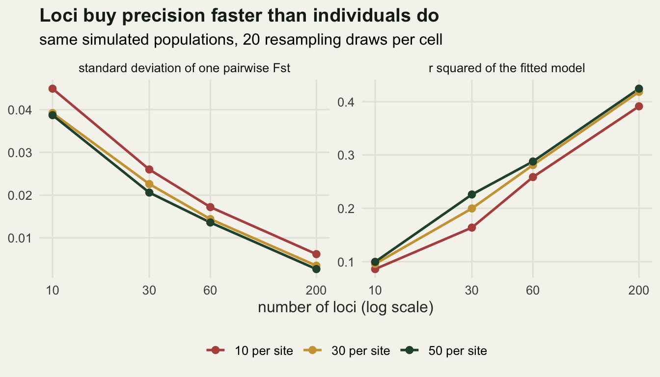

Figure 4: Standard deviation of one pairwise Fst estimate and r squared of the fitted model, against the number of loci, for three sample sizes per site.

The honest limit

The four checks constrain an analysis; they do not validate it. Between them they say how much evidence you have, whether the design can separate two explanations, whether the timescales match, and whether the response is measured well enough. All four are internal: they use only the data and the design, and they can all pass on a study whose conclusion is wrong.

Two failure modes survive every internal check. The first is non-equilibrium, and check 3 shows it cuts both ways: a real barrier can be invisible while a removed one is still printed in the data, and nothing in the fitted model separates either case from a landscape in balance. The second is the unmeasured variable. A resistance surface built from land cover cannot represent a disease front, a historical translocation, or a habitat type nobody mapped, and a confounder of that kind gives a well-fitting model with the wrong cause.

Neither is fixable from inside the analysis. The fixes are design and independent data: sample so the confounding breaks, which is check 2 turned into a field protocol, and bring in something the genetic distances do not contain, such as direct observations of movement, or samples from two time periods so the rate of change is measured rather than assumed.

Where to go next

This closes the landscape genetics cluster. The connectivity side of the argument has its own checking tutorial, which calibrates resistance distance against the random walk it claims to summarise and measures how much of a corridor map the arbitrary choices decide.

References

Landguth EL, Cushman SA, Schwartz MK, McKelvey KS, Murphy M, Luikart G 2010 Molecular Ecology 19(19):4179-4191 (10.1111/j.1365-294X.2010.04808.x)

Cushman SA, Landguth EL 2010 Molecular Ecology 19(17):3592-3602 (10.1111/j.1365-294X.2010.04656.x)

Hutchison DW, Templeton AR 1999 Evolution 53(6):1898-1914 (10.1111/j.1558-5646.1999.tb04571.x)

Prunier JG, Colyn M, Legendre X, Nimon KF, Flamand MC 2015 Molecular Ecology 24(2):263-283 (10.1111/mec.13029)

Related tutorials

• Isolation by distance and by resistance
• Multiple matrix regression with MMRR
• Optimising a resistance surface
• Checking a connectivity analysis