library(ggplot2)

te_pal <- list(forest = "#275139", green = "#2f8f63", sage = "#93a87f",
               clay = "#b5534e", gold = "#cda23f", line = "#dad9ca",
               ink = "#16241d", paper = "#f5f4ee")

theme_te <- function() {
  theme_minimal(base_size = 12) +
    theme(panel.grid.minor = element_blank(),
          panel.grid.major = element_line(colour = "#e7e6dc"),
          plot.background = element_rect(fill = "#f5f4ee", colour = NA),
          panel.background = element_rect(fill = "#f5f4ee", colour = NA),
          plot.title = element_text(face = "bold", colour = te_pal$ink),
          axis.title = element_text(colour = "#2c3a31"))
}Optimising a resistance surface
R
landscape genetics
model selection
ecology tutorial
ggplot2
Search land-cover resistance values against genetic distance in R, then measure how much optimised r squared a deliberately meaningless map already buys.
A resistance surface needs a number for every land-cover class, and nobody has that number. What a motorway costs a ground beetle is not written down anywhere, so the values get assigned by expert opinion, by a habitat model with no movement data behind it, or by whatever looked defensible at the time. The standard alternative is to let the genetic data choose: try many sets of values, compute the resistance distances each set implies, fit genetic distance against them, and keep the set that fits best.
The procedure works, in the sense that it always returns a best-fitting surface and the fit is usually good. This tutorial builds it on simulated data where the true resistances are known, then measures the two things the fit statistic does not report: how many other surfaces fit almost as well, and how well a map containing no information at all would have fitted after the same optimisation.
The lattice and the truth
Four hundred demes sit on a 20 by 20 lattice. Three land-cover classes are laid out as coherent patches by smoothing a random field and cutting it at its terciles, and the true resistances are 1, 5 and 50. Gene flow runs between rook neighbours only, at a rate proportional to the edge conductance 2 / (r_i + r_j), the conductance convention circuit theory uses: cheap ground on both sides of an edge means a well connected edge.
smooth_field <- function(n, passes, seed) {
  set.seed(seed)
  z <- matrix(runif(n * n), n, n)
  for (p in seq_len(passes)) {
    pad <- rbind(z[1, ], z, z[n, ])
    pad <- cbind(pad[, 1], pad, pad[, n])
    z <- (pad[1:n, 2:(n + 1)] + pad[3:(n + 2), 2:(n + 1)] +
            pad[2:(n + 1), 1:n] + pad[2:(n + 1), 3:(n + 2)] +
            4 * pad[2:(n + 1), 2:(n + 1)]) / 8
  }
  (z - min(z)) / (max(z) - min(z))
}

class_map <- function(field) {
  cuts <- quantile(field, c(1 / 3, 2 / 3))
  matrix(1L + (field > cuts[1]) + (field > cuts[2]),
         nrow(field), ncol(field))
}

nn <- 20
n_deme <- nn * nn
idx <- matrix(seq_len(n_deme), nn, nn)
ii <- c(as.vector(idx[-nn, ]), as.vector(idx[, -nn]))
jj <- c(as.vector(idx[-1, ]), as.vector(idx[, -1]))

conductance <- function(res) 2 / (res[ii] + res[jj])

laplacian <- function(res) {
  cnd <- conductance(res)
  lap <- matrix(0, n_deme, n_deme)
  lap[cbind(ii, jj)] <- -cnd
  lap[cbind(jj, ii)] <- -cnd
  diag(lap) <- -rowSums(lap)
  lap
}

res_dist <- function(res, nodes) {
  lap <- laplacian(res)
  keep <- setdiff(seq_len(n_deme), nodes[1])
  pos <- match(nodes[-1], keep)
  rhs <- matrix(0, length(keep), length(nodes) - 1)
  rhs[cbind(pos, seq_along(pos))] <- 1
  inv_red <- solve(lap[keep, keep], rhs)
  inv <- matrix(0, length(nodes), length(nodes))
  inv[-1, -1] <- inv_red[pos, ]
  dg <- diag(inv)
  outer(dg, dg, "+") - 2 * inv
}
Effective resistance between two nodes is R_ij = L+_ii + L+_jj - 2 L+_ij, with L+ the pseudo-inverse of the graph Laplacian. The full pseudo-inverse is never needed. Grounding one node and inverting the reduced Laplacian gives the same pairwise answers, and because only sixteen demes are ever sampled, one solve() with fifteen right hand sides per surface is enough. That economy is what makes the rest of the tutorial affordable, because the searches below repeat it about a thousand times in all.
cls_true <- class_map(smooth_field(nn, 6, seed = 5311))
r_true <- c(1, 5, 50)
res_true <- matrix(r_true[cls_true], nn, nn)

same_class <- function(cm) mean(cm[ii] == cm[jj])
cat("lattice:", nn, "by", nn, " demes:", n_deme,
    " rook edges:", length(ii), "\n")
lattice: 20 by 20 demes: 400 rook edges: 760 cat("cells per class:", as.integer(table(cls_true)), "\n")cells per class: 134 133 133 cat("share of neighbour pairs in the same class:",
round(same_class(cls_true), 4), "\n")share of neighbour pairs in the same class: 0.6816 cat("edge conductance from best to worst:",
round(range(conductance(res_true)), 4), "\n")edge conductance from best to worst: 0.02 1 The three classes cover roughly equal shares of the lattice, and the smoothing leaves them as coherent patches rather than speckle. The best edge is fifty times more conductive than the worst, which is a strong landscape effect by the standards of published studies.
n_loci <- 60
n_dip <- 50
gens <- 300
m_scale <- 0.1

mig <- matrix(0, n_deme, n_deme)
mig[cbind(ii, jj)] <- m_scale * conductance(res_true)
mig[cbind(jj, ii)] <- m_scale * conductance(res_true)
diag(mig) <- 1 - rowSums(mig)
cat("largest total emigration rate:", round(1 - min(diag(mig)), 4),
    " smallest:", round(1 - max(diag(mig)), 5), "\n")
largest total emigration rate: 0.4 smallest: 0.00564 set.seed(5312)
freq <- matrix(0.5, n_loci, n_deme)
for (g in seq_len(gens)) {
freq <- freq %*% mig
freq <- matrix(rbinom(length(freq), 2 * n_dip, as.vector(freq)),
n_loci) / (2 * n_dip)
}
set.seed(5313)
sites <- sort(sample(n_deme, 16))
sampled <- freq[, sites]
is_poly <- apply(sampled, 1, function(x) any(x > 0) && any(x < 1))
sampled <- sampled[is_poly, , drop = FALSE]
cat("sampled demes per class:", as.integer(table(cls_true[sites])),
" loci still polymorphic in the sample:", sum(is_poly), "\n")sampled demes per class: 6 7 3 loci still polymorphic in the sample: 60 fst_matrix <- function(pm) {
k <- ncol(pm)
out <- matrix(0, k, k)
for (a in seq_len(k - 1)) {
for (b in (a + 1):k) {
p_bar <- (pm[, a] + pm[, b]) / 2
hs <- (2 * pm[, a] * (1 - pm[, a]) + 2 * pm[, b] * (1 - pm[, b])) / 2
ht <- 2 * p_bar * (1 - p_bar)
out[a, b] <- out[b, a] <- mean(ht - hs) / mean(ht)
}
}
out
}
fst <- fst_matrix(sampled)
up <- which(upper.tri(fst))
lin_fst <- fst[up] / (1 - fst[up])
cat("pairs:", length(up), " Fst from", round(min(fst[up]), 4), "to",
round(max(fst[up]), 4), " mean", round(mean(fst[up]), 4), "\n")pairs: 120 Fst from 0.0195 to 0.3779 mean 0.1053 cat("linearised Fst from", round(min(lin_fst), 4), "to",
round(max(lin_fst), 4), "\n")linearised Fst from 0.0198 to 0.6074 Allele frequencies move by migration and then by binomial drift, vectorised so that all 60 loci advance together. Emigration is fastest on the cheapest ground and slowest inside the expensive class, and after 300 generations the sixteen sampled demes give 120 pairwise Fst values from 0.0195 to 0.3779, averaging 0.1053. Linearising as Fst / (1 - Fst) takes the largest pair to 0.6074. No locus went monomorphic across the sample, so all 60 contribute.
land_df <- data.frame(x = rep(seq_len(nn), each = nn),
                      y = rep(seq_len(nn), times = nn),
                      cover = factor(as.vector(cls_true), levels = 1:3,
                        labels = c("class 1, resistance 1",
                                   "class 2, resistance 5",
                                   "class 3, resistance 50")))
site_df <- data.frame(x = ((sites - 1) %/% nn) + 1,
                      y = ((sites - 1) %% nn) + 1)

ggplot(land_df, aes(x, y)) +
  geom_raster(aes(fill = cover)) +
  geom_point(data = site_df, shape = 21, fill = te_pal$clay,
             colour = "white", size = 3, stroke = 0.8) +
  coord_equal() +
  scale_fill_manual(values = c(te_pal$sage, te_pal$green, te_pal$forest),
                    name = NULL) +
  labs(title = "Land cover and the sampled demes",
       subtitle = "the resistance values are the truth the search has to find",
       x = NULL, y = NULL) +
  theme_te() +
  theme(axis.text = element_blank(), panel.grid = element_blank(),
        legend.position = "bottom")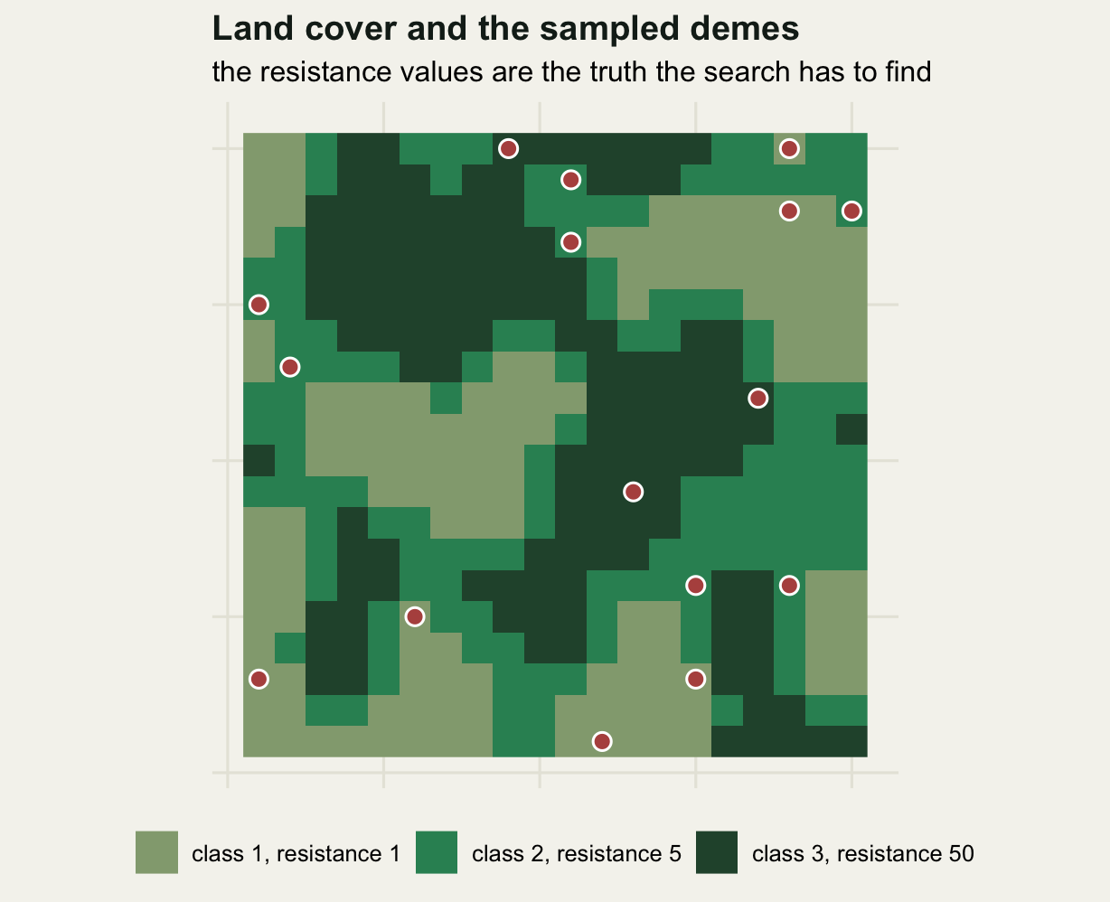
The sampled demes fall unevenly across the three classes, as the counts above show. That imbalance is what random sampling of a patchy landscape gives, and it already limits how much the data can say about the least-sampled class.
Only ratios are identified
One property of the model deserves a measurement rather than a footnote. Multiplying every cell’s resistance by a constant multiplies every edge resistance by the same constant, so every effective resistance is multiplied by it too, and a straight-line fit cannot see a change of units in its predictor.
rd_one <- res_dist(res_true, sites)[up]
rd_seven <- res_dist(7 * res_true, sites)[up]
cat("ratio of resistance distances after scaling every cell by seven:",
    round(range(rd_seven / rd_one), 10), "\n")
ratio of resistance distances after scaling every cell by seven: 7 7 cat("r squared before scaling:", round(cor(lin_fst, rd_one)^2, 4),
" after:", round(cor(lin_fst, rd_seven)^2, 4), "\n")r squared before scaling: 0.8346 after: 0.8346 Scaling every cell by seven multiplies all 120 pairwise resistance distances by exactly 7, to ten decimal places, and the r squared is 0.8346 either way. The search therefore has three unknowns but only two directions to move in, which is why class 1 is pinned at 1 from here on. It also settles what the answer can mean: a statement about an absolute resistance value is a statement about an arbitrary scale, and only the ratios between classes are being estimated.
Searching the grid
Class 2 and class 3 get a nine-point logarithmic grid from 1 to 300, giving 81 candidate surfaces. Each one needs its own Laplacian and its own decomposition; the pairwise resistance distances are kept because the cross-validation below reuses them.
gv <- exp(seq(0, log(300), length.out = 9))
cand <- expand.grid(i2 = seq_len(9), i3 = seq_len(9))

timing <- system.time({
  rd_store <- matrix(NA_real_, nrow(cand), length(up))
  for (k in seq_len(nrow(cand))) {
    rr <- c(1, gv[cand$i2[k]], gv[cand$i3[k]])
    rd_store[k, ] <- res_dist(matrix(rr[cls_true], nn, nn), sites)[up]
  }
})
cand$r2 <- apply(rd_store, 1, function(z) cor(lin_fst, z)^2)

cat("candidate surfaces:", nrow(cand), " Laplacian solves:", nrow(cand),
    " elapsed seconds:", round(timing[["elapsed"]], 1), "\n")
candidate surfaces: 81 Laplacian solves: 81 elapsed seconds: 0.9 cat("grid values:", round(gv, 2), "\n")grid values: 1 2.04 4.16 8.49 17.32 35.33 72.08 147.06 300 best <- cand[which.max(cand$r2), ]
cat("best fit at class 2 =", round(gv[best$i2], 2), "and class 3 =",
round(gv[best$i3], 2), "with r squared", round(best$r2, 4), "\n")best fit at class 2 = 8.49 and class 3 = 300 with r squared 0.8858 cat("r squared at the true surface (5 and 50):",
round(cor(lin_fst, rd_one)^2, 4),
" at a surface with no landscape in it:",
round(cand$r2[cand$i2 == 1 & cand$i3 == 1], 4), "\n")r squared at the true surface (5 and 50): 0.8346 at a surface with no landscape in it: 0.0306 The best-fitting surface puts class 2 at 8.49 and class 3 at 300, with an r squared of 0.8858. Class 2 lands at 1.7 times its true value of 5. Class 3 is not close to 50; it is pinned at the top of the searched range, which means the data would have taken a larger number if the grid had offered one.
Two other numbers belong next to it. The true surface, the one the genetic data were actually generated from, scores 0.8346, lower than the best-fitting wrong surface by 0.0512. A surface with no landscape in it at all, every class costing 1 so that resistance distance is pure lattice geometry, scores 0.0306. The landscape therefore carries nearly all of the signal here, and the optimiser still prefers a surface that puts class 3 at 6.0 times its true value, the class that matters most.
step <- log(300) / 8
surf_df <- data.frame(x = log(gv[cand$i2]), y = log(gv[cand$i3]), r2 = cand$r2)
ridge_df <- surf_df[cand$r2 >= max(cand$r2) - 0.005, ]
mark_df <- data.frame(x = log(c(5, gv[best$i2])),
                      y = log(c(50, gv[best$i3])),
                      what = c("true surface", "best fit"))
brk <- c(1, 3, 10, 30, 100, 300)

ggplot(surf_df, aes(x, y)) +
  geom_tile(aes(fill = r2), width = step, height = step) +
  geom_tile(data = ridge_df, fill = NA, colour = te_pal$gold,
            width = step, height = step, linewidth = 0.7) +
  geom_point(data = mark_df, aes(shape = what), colour = te_pal$clay,
             size = 4, stroke = 1.2) +
  scale_fill_gradient(low = te_pal$paper, high = te_pal$forest,
                      name = "r squared") +
  scale_shape_manual(values = c(`true surface` = 4, `best fit` = 1),
                     name = NULL) +
  scale_x_continuous(breaks = log(brk), labels = brk) +
  scale_y_continuous(breaks = log(brk), labels = brk) +
  labs(title = "The fit is a ridge, not a peak",
       subtitle = "gold outline: within 0.005 of the best r squared",
       x = "resistance of class 2 (log scale)",
       y = "resistance of class 3 (log scale)") +
  theme_te()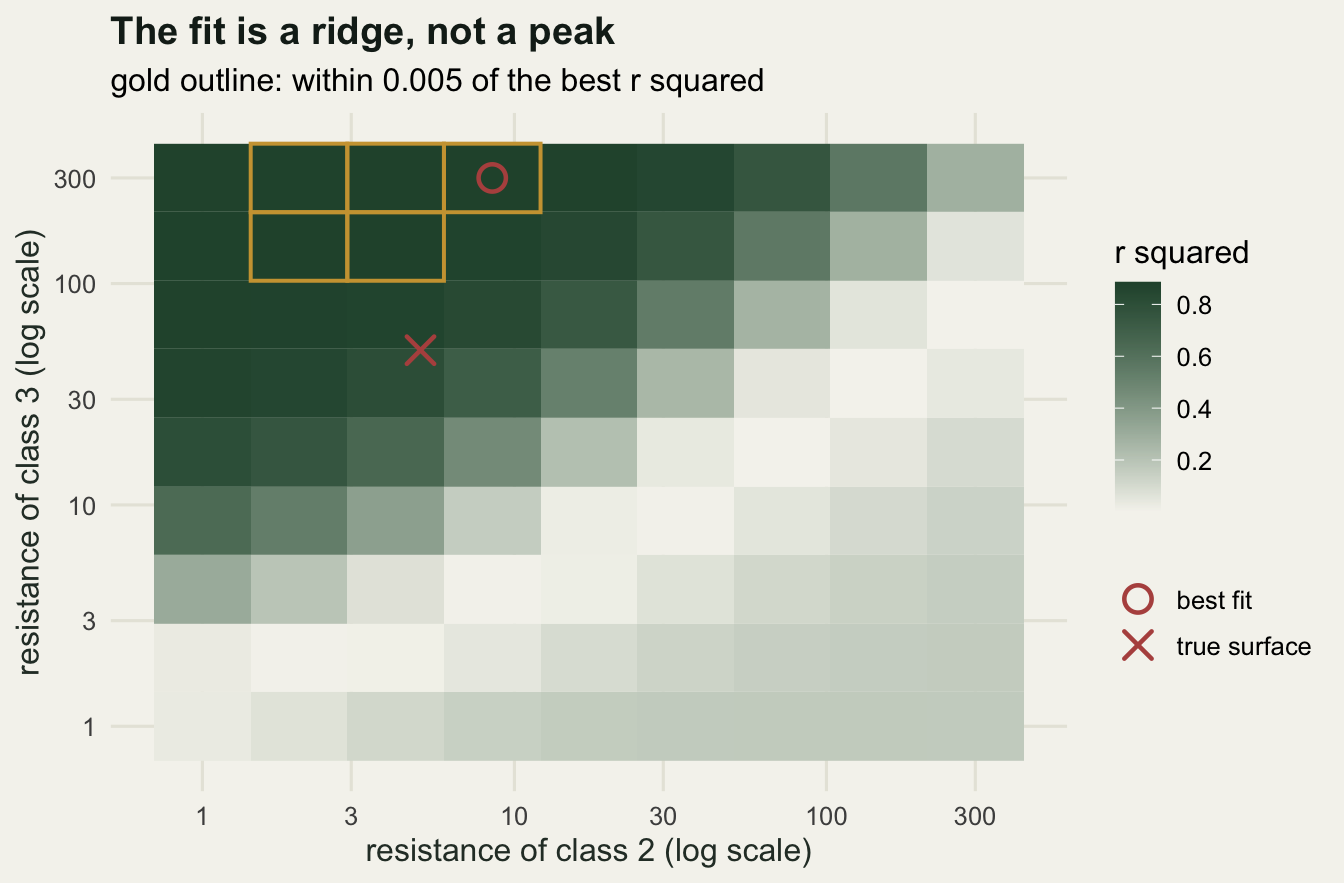
How wide is the ridge
The picture is a ridge running up the left of the grid, so the useful question is not where the maximum is but how flat the top is.
ridge <- cand[cand$r2 >= max(cand$r2) - 0.005, ]
cat("grid cells within 0.005 of the best r squared:", nrow(ridge), "of",
    nrow(cand), "\n")
grid cells within 0.005 of the best r squared: 5 of 81 cat("class 2 values in that set:", round(range(gv[ridge$i2]), 2),
" class 3 values:", round(range(gv[ridge$i3]), 2), "\n")class 2 values in that set: 2.04 8.49 class 3 values: 147.06 300 cat("r squared across that set:", round(range(ridge$r2), 4), "\n")r squared across that set: 0.8813 0.8858 cat("penalty for using the true surface instead of the best grid point:",
round(max(cand$r2) - cor(lin_fst, rd_one)^2, 4), "\n")penalty for using the true surface instead of the best grid point: 0.0512 Only 5 of the 81 cells sit within 0.005 of the best r squared, spanning 0.8813 to 0.8858. Inside that set class 2 ranges from 2.04 to 8.49 and class 3 from 147.06 to 300. In words: the data pin class 2 only to within a factor of 4.2, and they place no upper bound at all on class 3 within the range searched. Anyone reporting the maximum as an estimate would write down 8.49 and 300 and imply three significant figures of knowledge about a quantity the data constrain only to that window in one direction and not at all in the other.
The boundary result deserves saying plainly, because it recurs in real analyses. A search that stops at 300 reports 300. The reported optimum is partly a description of where the analyst stopped looking, and the only way to notice is to widen the range and see whether the answer moves with it.
What an optimised fit is worth
An r squared of 0.8858 sounds like strong support for the surface. The question that turns it into evidence is what the same procedure would have produced from a map with nothing in it. Keep the genetic data exactly as they are, generate fresh three-class maps from new random fields with the same patch scale and the same class proportions, and run the same optimisation on each. To keep the run affordable the null uses every second grid value, so 25 surfaces per map instead of 81; the first line below reports what that coarsening costs on the true map, so the tilt can be read off rather than assumed.
sub_i <- c(1, 3, 5, 7, 9)
sub_cand <- expand.grid(i2 = sub_i, i3 = sub_i)
on_sub <- cand$i2 %in% sub_i & cand$i3 %in% sub_i
cat("best r squared on the true map, full grid:", round(max(cand$r2), 4),
    " on the coarse subgrid:", round(max(cand$r2[on_sub]), 4), "\n")
best r squared on the true map, full grid: 0.8858 on the coarse subgrid: 0.8847 set.seed(5314)
null_seeds <- sample(100000, 40)
null_tim <- system.time({
null_best <- numeric(length(null_seeds))
null_same <- numeric(length(null_seeds))
for (s in seq_along(null_seeds)) {
cm <- class_map(smooth_field(nn, 6, seed = null_seeds[s]))
null_same[s] <- same_class(cm)
top <- 0
for (k in seq_len(nrow(sub_cand))) {
rr <- c(1, gv[sub_cand$i2[k]], gv[sub_cand$i3[k]])
rd <- res_dist(matrix(rr[cm], nn, nn), sites)[up]
top <- max(top, cor(lin_fst, rd)^2)
}
null_best[s] <- top
}
})
cat("meaningless maps:", length(null_best), " surfaces searched each:",
nrow(sub_cand), " elapsed seconds:", round(null_tim[["elapsed"]], 1), "\n")meaningless maps: 40 surfaces searched each: 25 elapsed seconds: 9.2 cat("mean share of neighbour pairs in the same class, meaningless maps:",
round(mean(null_same), 4), " true map:", round(same_class(cls_true), 4),
"\n")mean share of neighbour pairs in the same class, meaningless maps: 0.675 true map: 0.6816 cat("optimised r squared on meaningless maps: mean", round(mean(null_best), 4),
" median", round(median(null_best), 4),
" 95th percentile", round(quantile(null_best, 0.95)[[1]], 4),
" max", round(max(null_best), 4), "\n")optimised r squared on meaningless maps: mean 0.1535 median 0.1282 95th percentile 0.4285 max 0.4899 cat("meaningless maps beating the true map:",
sum(null_best >= max(cand$r2[on_sub])), "\n")meaningless maps beating the true map: 0 The reshuffled maps are matched to the real one on the property that matters for this test: they come from the same smoothing and the same tercile cut, and the chunk prints the share of neighbouring cell pairs sharing a class for both, so they are equally patchy and differ only in where the patches are.
Optimising resistance values on those maps gives a mean r squared of 0.1535, a 95th percentile of 0.4285 and a maximum of 0.4899. That maximum came from a map drawn without any reference to the genetic data, then tuned until it fitted. It is the reason an optimised fit statistic cannot be read on its own scale: fitting two free values to 120 correlated pairwise distances buys a substantial r squared from geometry alone, and the amount it buys is not something you can guess.
null_df <- data.frame(r2 = null_best)

ggplot(null_df, aes(r2)) +
  geom_histogram(binwidth = 0.05, boundary = 0, fill = te_pal$sage,
                 colour = "white") +
  geom_vline(xintercept = max(cand$r2), colour = te_pal$clay, linewidth = 1) +
  geom_vline(xintercept = cand$r2[cand$i2 == 1 & cand$i3 == 1],
             colour = te_pal$gold, linewidth = 1, linetype = "dashed") +
  scale_y_continuous(breaks = seq(0, 12, 3)) +
  coord_cartesian(xlim = c(0, 0.92)) +
  labs(title = "What an optimised fit buys on a meaningless map",
       subtitle = "forty reshuffled maps; red line: the true map, dashed: no landscape",
       x = "best r squared after optimising the resistance values",
       y = "number of maps") +
  theme_te()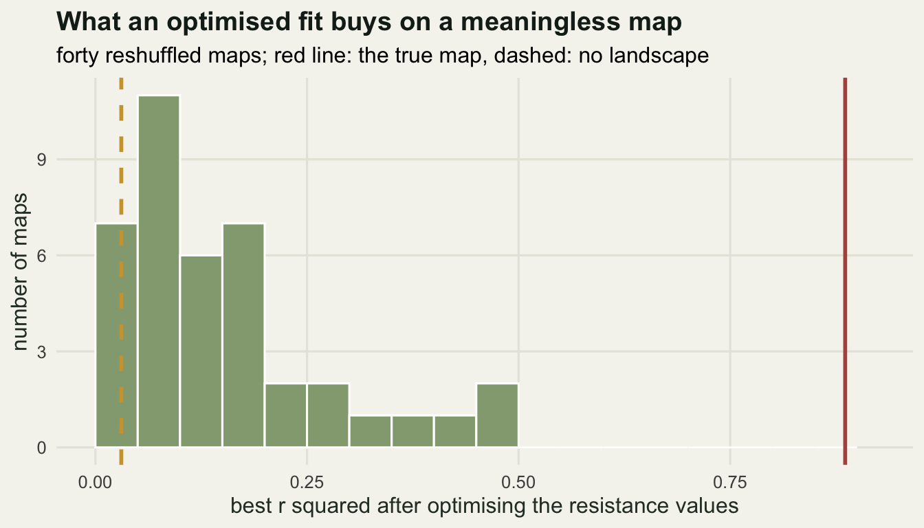
The comparison also comes out well here, and that is worth stating as clearly as the warning. None of the 40 reshuffled maps came near the 0.8847 the true map reaches on that same coarse subgrid, so on these data the exercise is informative: the surface is doing work that a patchy map of the right texture in the wrong places cannot do. That is the condition under which optimising a resistance surface tells you something, and it is a condition to demonstrate rather than assume, because the same code run on a weaker landscape effect or fewer loci would put the true map inside its own null.
Holding out demes
The remaining worry is that the surface was chosen using the same 120 pairs it is then judged on. Splitting pairs at random does not help, because a held-out pair shares both of its demes with training pairs. Holding out demes is the least leaky split available: refit the search on the pairs among the retained demes, then look at the pairs among the held-out demes only.
set.seed(5315)
fold <- sample(rep(1:4, each = 4))
pair_a <- row(fst)[up]
pair_b <- col(fst)[up]

cv <- NULL
held_obs <- NULL
held_pred <- NULL
for (f in 1:4) {
  train <- !(fold[pair_a] == f | fold[pair_b] == f)
  test <- fold[pair_a] == f & fold[pair_b] == f
  tr_r2 <- apply(rd_store, 1, function(z) cor(lin_fst[train], z[train])^2)
  pick <- which.max(tr_r2)
  fit <- lm(lin_fst[train] ~ rd_store[pick, train])
  pred <- coef(fit)[[1]] + coef(fit)[[2]] * rd_store[pick, test]
  held_obs <- c(held_obs, lin_fst[test])
  held_pred <- c(held_pred, pred)
  cv <- rbind(cv, data.frame(fold = f, train_pairs = sum(train),
                             held_pairs = sum(test),
                             class2 = round(gv[cand$i2[pick]], 1),
                             class3 = round(gv[cand$i3[pick]], 1),
                             train_r2 = round(tr_r2[pick], 4),
                             held_r2 = round(cor(lin_fst[test],
                                                 rd_store[pick, test])^2, 4)))
}
print(cv, row.names = FALSE)
fold train_pairs held_pairs class2 class3 train_r2 held_r2
1 66 6 8.5 300 0.8854 0.5416
2 66 6 8.5 300 0.8602 0.9588
3 66 6 1.0 300 0.9271 0.7801
4 66 6 8.5 300 0.8841 0.7657cat("mean in-sample r squared:", round(mean(cv$train_r2), 4),
" mean held-out squared correlation:", round(mean(cv$held_r2), 4), "\n")mean in-sample r squared: 0.8892 mean held-out squared correlation: 0.7615 pooled <- 1 - sum((held_obs - held_pred)^2) /
sum((held_obs - mean(held_obs))^2)
cat("pooled held-out pairs:", length(held_obs),
" predictive r squared using the training fit:", round(pooled, 4), "\n")pooled held-out pairs: 24 predictive r squared using the training fit: 0.8213 Each fold trains on 66 pairs and is tested on the 6 pairs among its four held-out demes. Mean in-sample r squared is 0.8892 and the mean held-out squared correlation is 0.7615; pooling the 24 held-out pairs and using each fold’s own fitted line to predict them gives a predictive r squared of 0.8213. The surface still predicts demes it was not fitted on, but the held-out average sits below the in-sample one and the per-fold values swing widely, from 0.5416 to 0.9588, the top of that range sitting above the in-sample 0.8602 of the fold that produced it.
Class 3 sat at 300 in 4 of the four folds, and class 2 at the full-data optimum of 8.49 in 3 of the four. That is the informative part of the table rather than a reassurance. The less the fold values move when a quarter of the demes are dropped, the less power the hold-out has to reject the surface. The held-out pairs also sit in the same landscape, inherit the same drift history, and were sampled in the same campaign as the training pairs, so this is a check on whether the fit survives new pairs, not on whether the surface would survive a new study area.
The honest limits
The circularity is the deep problem and no amount of resampling removes it. The resistance values are estimated from the same genetic distances used to score them, so “the genetic data support this surface” is close to vacuous unless a null and a hold-out are reported alongside it. The measurements above give the shape of the correction: a meaningless map bought up to 0.4899 here, which is the level below which an optimised r squared says nothing.
Only ratios are identified, and within the ratios the ridge is wide. A published value such as “resistance 50 for roads” carries far less information than its precision suggests, and when the optimum sits at the edge of the searched grid, as it does here, the number is partly a report on the grid. Publishing the ridge, or at least the set of values within a small distance of the best fit, costs one extra figure and prevents a false reading.
Nothing here validates the underlying model. Effective resistance assumes gene flow behaves like a random walk on a resistor network, and the search only ever compares members of that family against each other. A better fit inside a wrong family is still a wrong family, and the fit statistic cannot see the difference.
Where to go next
The next tutorial in this cluster collects the checks that a landscape genetics analysis needs before its map is believed: how many loci and how many sites the genetic distances require, what a permutation test can and cannot rule out, how sampling design decides which landscape hypotheses are even separable, and which of the diagnostics here transfer to real data where no truth is available.
References
Peterman WE 2018 Methods in Ecology and Evolution 9(6):1638-1647 (10.1111/2041-210X.12984)
Graves TA, Beier P, Royle JA 2013 Molecular Ecology 22(15):3888-3903 (10.1111/mec.12348)
Zeller KA, McGarigal K, Whiteley AR 2012 Landscape Ecology 27(6):777-797 (10.1007/s10980-012-9737-0)
Shirk AJ, Wallin DO, Cushman SA, Rice CG, Warheit KI 2010 Molecular Ecology 19(17):3603-3619 (10.1111/j.1365-294X.2010.04745.x)